Back
BackProblem 10.1.3a
Notation The author conducted an experiment in which the height of each student was measured in centimeters and those heights were matched with the same students’ scores on the first statistics test.
a. For this sample of paired data, what does r represent, and what does represent?
Problem 10.1.1b
Notation The author conducted an experiment in which the height of each student was measured in centimeters and those heights were matched with the same students’ scores on the first statistics test.
b. Without doing any research or calculations, estimate the value of r.
Problem 10.1.1c
Notation The author conducted an experiment in which the height of each student was measured in centimeters and those heights were matched with the same students’ scores on the first statistics test.
c. Does r change if the heights are converted from centimeters to inches?
Problem 10.1.2
Notation The author conducted an experiment in which the height of each student was measured in centimeters and those heights were matched with the same students’ scores on the first statistics test. If we find that r = 0, does that indicate that there is no association between those two variables?
Problem 10.1.11a
Explore!
Exercises 11 and 12 provide two data sets from “Graphs in Statistical Analysis,” by F. J. Anscombe, the American Statistician, Vol. 27. For each exercise,
a. Construct a scatterplot.
Problem 10.1.9b
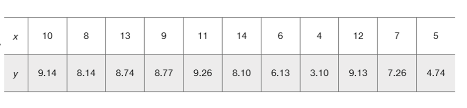
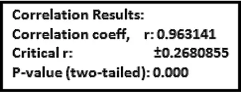
Outlier Refer to the accompanying Minitab-generated scatterplot.
b. After identifying the 10 pairs of coordinates corresponding to the 10 points, find the value of the correlation coefficient r and determine whether there is a linear correlation.
Problem 10.1.10a
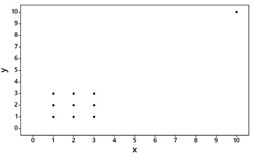
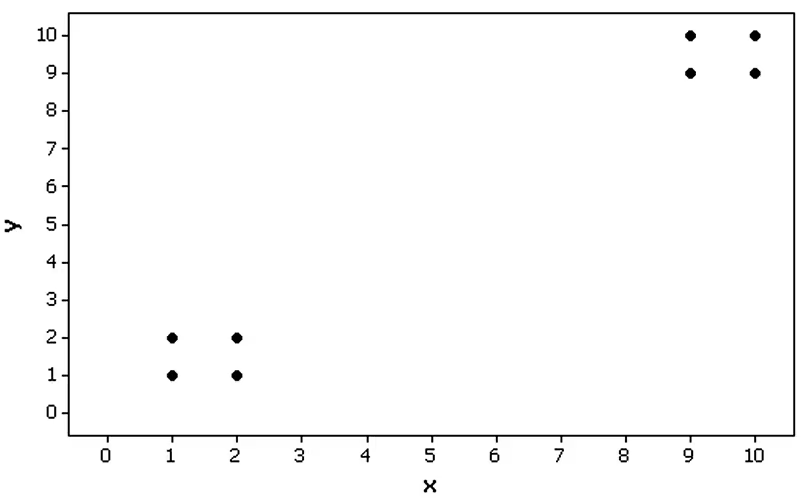
Clusters Refer to the Minitab-generated scatterplot. The four points in the lower left corner are measurements from women, and the four points in the upper right corner are from men.
a. Examine the pattern of the four points in the lower left corner (from women) only, and subjectively determine whether there appears to be a correlation between x and y for women.
Problem 10.1.10d
Clusters Refer to the Minitab-generated scatterplot. The four points in the lower left corner are measurements from women, and the four points in the upper right corner are from men.
Find the value of the linear correlation coefficient using all eight points. What does that value suggest about the relationship between x and y?
Problem 10.1.5
Interpreting r
In Exercises 5–8, use a significance level of α = 0.05 and refer to the accompanying displays.
Bear Weight and Chest Size Fifty-four wild bears were anesthetized, and then their weights and chest sizes were measured and listed in Data Set 18 “Bear Measurements” in Appendix B; results are shown in the accompanying Statdisk display. Is there sufficient evidence to support the claim that there is a linear correlation between the weights of bears and their chest sizes? When measuring an anesthetized bear, is it easier to measure chest size than weight? If so, does it appear that a measured chest size can be used to predict the weight?
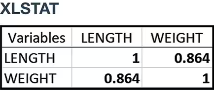
Problem 10.1.6
Interpreting r
In Exercises 5–8, use a significance level of α = 0.05 and refer to the accompanying displays.
Bear Length and Weight The lengths (inches) and weights (pounds) of 54 bears are obtained from Data Set 18 “Bear Measurements” in Appendix B, and results are shown in the accompanying XLSTAT display. Is there sufficient evidence to support the claim that there is a linear correlation between length and weight?
Problem 10.1.15
Testing for a Linear Correlation
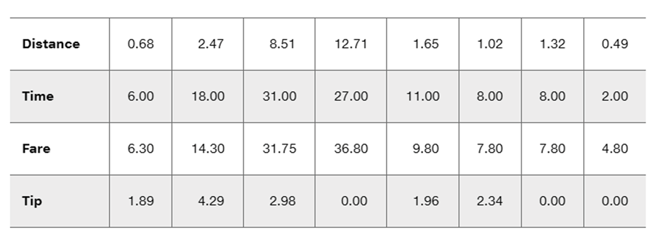
In Exercises 13–28, construct a scatterplot, and find the value of the linear correlation coefficient r. Also find the P-value or the critical values of r from Table A-6. Use a significance level of α = 0.05. Determine whether there is sufficient evidence to support a claim of a linear correlation between the two variables. (Save your work because the same data sets will be used in Section 10-2 exercises.)
Taxis The table below includes data from New York City taxi rides (from Data Set 32 “Taxis” in Appendix B). The distances are in miles, the times are in minutes, the fares are in dollars, and the tips are in dollars. Is there sufficient evidence to support the claim that there is a linear correlation between the time of the ride and the tip amount? Does it appear that riders base their tips on the time of the ride?
Problem 10.1.14
Testing for a Linear Correlation
In Exercises 13–28, construct a scatterplot, and find the value of the linear correlation coefficient r. Also find the P-value or the critical values of r from Table A-6. Use a significance level of α = 0.05. Determine whether there is sufficient evidence to support a claim of a linear correlation between the two variables. (Save your work because the same data sets will be used in Section 10-2 exercises.)
Powerball Jackpots and Tickets Sold Listed below are the same data from Table 10-1 in the Chapter Problem, but an additional pair of values has been added from actual Powerball results. Is there sufficient evidence to conclude that there is a linear correlation between lottery jackpots and numbers of tickets sold? Comment on the effect of the added pair of values in the last column. Compare the results to those obtained in Example 4.
Problem 10.1.29
Appendix B Data Sets
In Exercises 29–32, use the data from Appendix B to construct a scatterplot, find the value of the linear correlation coefficient r, and find either the P-value or the critical values of r from Table A-6 using a significance level of α = 0.05. Determine whether there is sufficient evidence to support the claim of a linear correlation between the two variables.
Taxis Repeat Exercise 15 using all of the time/tip data from the 703 taxi rides listed in Data Set 32 “Taxis” from Appendix B. Compare the results to those found in Exercise 15.
Problem 10.1.34
Randomization
For Exercises 33–36, repeat the indicated exercise using the resampling method of randomization.
Powerball Jackpots and Tickets Sold Exercise 14
Problem 10.1.16
Testing for a Linear Correlation
In Exercises 13–28, construct a scatterplot, and find the value of the linear correlation coefficient r. Also find the P-value or the critical values of r from Table A-6. Use a significance level of α = 0.05. Determine whether there is sufficient evidence to support a claim of a linear correlation between the two variables. (Save your work because the same data sets will be used in Section 10-2 exercises.)
Taxis Using the data from Exercise 15, is there sufficient evidence to support the claim that there is a linear correlation between the distance of the ride and the tip amount? Does it appear that riders base their tips on the distance of the ride?
Problem 10.1.17
Testing for a Linear Correlation
In Exercises 13–28, construct a scatterplot, and find the value of the linear correlation coefficient r. Also find the P-value or the critical values of r from Table A-6. Use a significance level of α = 0.05. Determine whether there is sufficient evidence to support a claim of a linear correlation between the two variables. (Save your work because the same data sets will be used in Section 10-2 exercises.)
Taxis Using the data from Exercise 15, is there sufficient evidence to support the claim that there is a linear correlation between the distance of the ride and the fare (cost of the ride)?
Problem 10.2.19
Regression and Predictions
Exercises 13–28 use the same data sets as Exercises 13–28 in Section 10-1.
Find the regression equation, letting the first variable be the predictor (x) variable.
Find the indicated predicted value by following the prediction procedure summarized in Figure 10-5.
Oscars Listed below are ages of recent Oscar winners matched by the years in which the awards were won (from Data Set 21 “Oscar Winner Age” in Appendix B). Find the best predicted age of an Oscar-winning actress given that the Oscar winner for best actor is 59 years of age. How does the result compare to the actual actress age of 60 years?
[IMAGE]
Problem 10.2.22
Regression and Predictions
Exercises 13–28 use the same data sets as Exercises 13–28 in Section 10-1.
Find the regression equation, letting the first variable be the predictor (x) variable.
Find the indicated predicted value by following the prediction procedure summarized in Figure 10-5.
Subway and the CPI Use the subway/CPI data from the preceding exercise. What is the best predicted value of the CPI when the subway fare is $3.00?
Problem 10.2.25
Regression and Predictions
Exercises 13–28 use the same data sets as Exercises 13–28 in Section 10-1.
Find the regression equation, letting the first variable be the predictor (x) variable.
Find the indicated predicted value by following the prediction procedure summarized in Figure 10-5.
Cars Sales and the Super Bowl Listed below are the annual numbers of cars sold (thousands) and the numbers of points scored in the Super Bowl that same year. What is the best predicted number of Super Bowl points in a year with sales of 8423 thousand cars? How close is the predicted number to the actual result of 37 points?
[IMAGE]
Problem 10.2.29
Large Data Sets
Exercises 29–32 use the same Appendix B data sets as Exercises 29–32 in Section 10-1. In each case, find the regression equation, letting the first variable be the predictor (x) variable. Find the indicated predicted values following the prediction procedure summarized in Figure 10-5.
Taxis Repeat Exercise 15 using all of the time/tip data from the 703 taxi rides listed in Data Set 32 “Taxis” from Appendix B.
Problem 10.2.30
Large Data Sets
Exercises 29–32 use the same Appendix B data sets as Exercises 29–32 in Section 10-1. In each case, find the regression equation, letting the first variable be the predictor (x) variable. Find the indicated predicted values following the prediction procedure summarized in Figure 10-5.
Taxis Repeat Exercise 16 using all of the distance/tip data from the 703 taxi rides listed in Data Set 32 “Taxis” from Appendix B.
Problem 10.2.33a
Least-Squares Property According to the least-squares property, the regression line minimizes the sum of the squares of the residuals. Refer to the jackpot/tickets data in Table 10-1 and use the regression equation y^ = -10.9 + 0.174x that was found in Examples 1 and 2 of this section.
a. Identify the nine residuals.
Problem 10.2.33b
Least-Squares Property According to the least-squares property, the regression line minimizes the sum of the squares of the residuals. Refer to the jackpot/tickets data in Table 10-1 and use the regression equation y^ = -10.9 + 0.174x that was found in Examples 1 and 2 of this section.
b. Find the sum of the squares of the residuals.
Problem 10.2.9
Finding the Equation of the Regression Line
In Exercises 9 and 10, use the given data to find the equation of the regression line. Examine the scatterplot and identify a characteristic of the data that is ignored by the regression line.
[IMAGE]
Problem 10.2.11a
Effects of an Outlier Refer to the Minitab-generated scatterplot given in Exercise 9 of Section 10-1
a. Using the pairs of values for all 10 points, find the equation of the regression line.
Problem 10.2.12a
Effects of Clusters Refer to the Minitab-generated scatterplot given in Exercise 10 of Section 10-1.
a. Using the pairs of values for all 8 points, find the equation of the regression line.
Problem 10.2.1a
Notation Using the weights (lb) and highway fuel consumption amounts (mi/gal) of the 48 cars listed in Data Set 35 “Car Data” of Appendix B, we get this regression equation:
y^ = 58.9 - 0.00749x, where x represents weight.
a. What does the symbol y^ represent?
Problem 10.2.1c
Notation Using the weights (lb) and highway fuel consumption amounts (mi/gal) of the 48 cars listed in Data Set 35 “Car Data” of Appendix B, we get this regression equation:
y^ = 58.9 - 0.00749x, where x represents weight.
c. What is the predictor variable?
Problem 10.2.2
Notation What is the difference between the regression equation y^ = b0 + b1x and the regression equation y = β0 + β1x.
Problem 10.2.3
Best-Fit Line
What is a residual?
In what sense is the regression line the straight line that “best” fits the points in a scatterplot?