Triola - Elementary Statistics 14th Edition

Ch. 10 - Correlation and Regression

Back

All textbooks

Triola 14th Edition

Ch. 10 - Correlation and Regression

Problem 10.5.16

Finding the Best Model

In Exercises 5–16, construct a scatterplot and identify the mathematical model that best fits the given data. Assume that the model is to be used only for the scope of the given data, and consider only linear, quadratic, logarithmic, exponential, and power models.

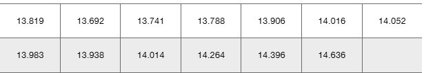
Global Warming Listed below are mean annual temperatures (°C) of the earth for each decade, beginning with the decade of the 1880s. Find the best model and then predict the value for 2090–2099. Comment on the result.

Problem 10.4.1

Response and Predictor Variables Using all of the Tour de France bicycle race results up to a recent year, we get this multiple regression equation: Speed = 29.2-0.00260Distance + 0.540Stages + 0.0570Finishers, where Speed is the mean speed of the winner (km/h), Distance is the length of the race (km), Stages is the number of stages in the race, and Finishers is the number of bicyclists who finished the race. Identify the response and predictor variables.

Problem 10.2.4

Correlation and Slope What is the relationship between the linear correlation coefficient r and the slope b1 of a regression line?

Problem 10.3.3

Coefficient of Determination Using the heights and weights described in Exercise 1, the linear correlation coefficient r is 0.394. Find the value of the coefficient of determination. What practical information does the coefficient of determination provide?

Problem 10.4.19

Dummy Variable Refer to Data Set 18 “Bear Measurements” in Appendix B and use the sex, age, and weight of the bears. For sex, let 0 represent female and let 1 represent male. Letting the response variable represent weight, use the variable of age and the dummy variable of sex to find the multiple regression equation. Use the equation to find the predicted weight of a bear with the characteristics given below. Does sex appear to have much of an effect on the weight of a bear?

Female bear that is 20 years of age

Male bear that is 20 years of age

Problem 10.3.11

Interpreting a Computer Display

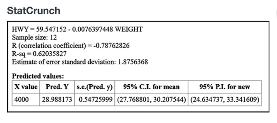
In Exercises 9–12, refer to the display obtained by using the paired data consisting of weights (pounds) and highway fuel consumption amounts (mi/gal) of the large cars included in Data Set 35 “Car Data” in Appendix B. Along with the paired weights and fuel consumption amounts, StatCrunch was also given the value of 4000 pounds to be used for predicting highway fuel consumption.

[IMAGE]

Predicting Highway Fuel Consumption Using a car weight of x = 4000 (pounds), what is the single value that is the best predicted amount of highway fuel consumption?

Problem 10.5.12

Finding the Best Model

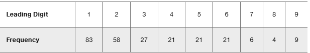
Detecting Fraud Leading digits of check amounts are often analyzed for the purpose of detecting fraud. The accompanying table lists frequencies of leading digits from checks written by the author (an honest guy).

Problem 10.3.4

Standard Error of Estimate A random sample of 118 different female statistics students is obtained and their weights are measured in kilograms and in pounds. Using the 118 paired weights (weight in kg, weight in lb), what is the value of se? For a female statistics student who weighs 100 lb, the predicted weight in kilograms is 45.4 kg. What is the 95% prediction interval?

Problem 10.5.4

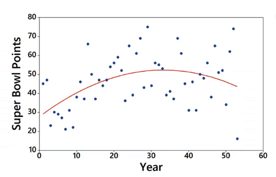
Interpreting a Graph The accompanying graph plots the numbers of points scored in each Super Bowl from the first Super Bowl in 1967 (coded as year 1) to the last Super Bowl at the time of this writing. The graph of the quadratic equation that best fits the data is also shown in red. What feature of the graph justifies the value of R^2 = 0.205 for the quadratic model?

Problem 10.5.11

Finding the Best Model

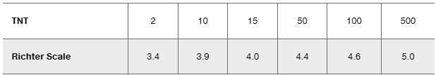
Richter Scale The table lists different amounts (metric tons) of the explosive TNT and the corresponding value measured on the Richter scale resulting from explosions of the TNT.

Problem 10.1.16

Testing for a Linear Correlation

In Exercises 13–28, construct a scatterplot, and find the value of the linear correlation coefficient r. Also find the P-value or the critical values of r from Table A-6. Use a significance level of α = 0.05. Determine whether there is sufficient evidence to support a claim of a linear correlation between the two variables. (Save your work because the same data sets will be used in Section 10-2 exercises.)

Taxis Using the data from Exercise 15, is there sufficient evidence to support the claim that there is a linear correlation between the distance of the ride and the tip amount? Does it appear that riders base their tips on the distance of the ride?

Problem 10.4.4

Interpreting R^2 For the multiple regression equation given in Exercise 1, we get R^2 = 0.897. What does that value tell us?

Problem 10.5.13

Finding the Best Model

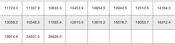
Stock Market Listed below in order by row are the annual high values of the Dow Jones Industrial Average for each year beginning with 2000. Find the best model and then predict the value for the last year listed. Is the predicted value close to the actual value of 26,828.4?

Problem 10.1.29

Appendix B Data Sets

In Exercises 29–32, use the data from Appendix B to construct a scatterplot, find the value of the linear correlation coefficient r, and find either the P-value or the critical values of r from Table A-6 using a significance level of α = 0.05. Determine whether there is sufficient evidence to support the claim of a linear correlation between the two variables.

Taxis Repeat Exercise 15 using all of the time/tip data from the 703 taxi rides listed in Data Set 32 “Taxis” from Appendix B. Compare the results to those found in Exercise 15.

Problem 10.4.17

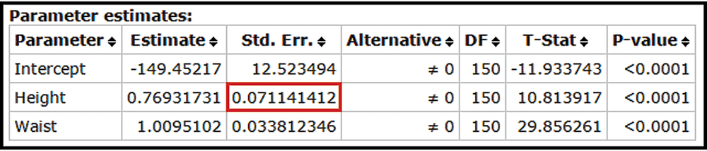
Testing Hypotheses About Regression Coefficients If the coefficient has a nonzero value, then it is helpful in predicting the value of the response variable. If it is not helpful in predicting the value of the response variable and can be eliminated from the regression equation. To test the claim that use the test statistic Critical values or P-values can be found using the t distribution with degrees of freedom, where k is the number of predictor variables and n is the number of observations in the sample. The standard error is often provided by software. For example, see the accompanying StatCrunch display for Example 1, which shows that (found in the column with the heading of “Std. Err.” and the row corresponding to the first predictor variable of height). Use the sample data in Data Set 1 “Body Data” and the StatCrunch display to test the claim that Also test the claim that What do the results imply about the regression equation?

Problem 10.2.3

Best-Fit Line

What is a residual?

In what sense is the regression line the straight line that “best” fits the points in a scatterplot?

Problem 10.5.15

Finding the Best Model

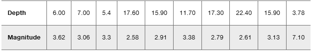
Earthquakes Listed below are earthquake depths (km) and magnitudes (Richter scale) of different earthquakes. Find the best model and then predict the magnitude for the last earthquake with a depth of 3.78 km. Is the predicted value close to the actual magnitude of 7.1?

Problem 10.3.15

Finding a Prediction Interval

In Exercises 13–16, use the following paired data consisting of weights of large cars (pounds) and highway fuel consumption (mi/gal) from Data Set 35 “Car Data” in Appendix B. (These are the same data used in Exercises 9-12.) Let x represent the weight of the car and let y represent the corresponding highway fuel consumption. Use the given weight and the given confidence level to construct a prediction interval estimate of highway fuel consumption.

Cars Use x = 3800 pounds with a 99% confidence level.

Problem 10.4.10

Garbage: Finding the Best Multiple Regression Equation

In Exercises 9–12, refer to the accompanying table, which was obtained by using the data from 62 households listed in Data Set 42 “Garbage Weight” in Appendix B. The response (y) variable is PLAS (weight of discarded plastic in pounds). The predictor (x) variables are METAL (weight of discarded metals in pounds), PAPER (weight of discarded paper in pounds), and GLASS (weight of discarded glass in pounds).

[IMAGE]

If exactly two predictor (x) variables are to be used to predict the weight of discarded plastic, which two variables should be chosen? Why?

Problem 10.2.25

Regression and Predictions

Exercises 13–28 use the same data sets as Exercises 13–28 in Section 10-1.

Find the regression equation, letting the first variable be the predictor (x) variable.

Find the indicated predicted value by following the prediction procedure summarized in Figure 10-5.

Cars Sales and the Super Bowl Listed below are the annual numbers of cars sold (thousands) and the numbers of points scored in the Super Bowl that same year. What is the best predicted number of Super Bowl points in a year with sales of 8423 thousand cars? How close is the predicted number to the actual result of 37 points?

[IMAGE]

Problem 10.1.2

Notation The author conducted an experiment in which the height of each student was measured in centimeters and those heights were matched with the same students’ scores on the first statistics test. If we find that r = 0, does that indicate that there is no association between those two variables?

Problem 10.1.34

Randomization

For Exercises 33–36, repeat the indicated exercise using the resampling method of randomization.

Powerball Jackpots and Tickets Sold Exercise 14

Problem 10.3.9

Interpreting a Computer Display

Testing for Correlation Use the information provided in the display to determine the value of the linear correlation coefficient. Is there sufficient evidence to support a claim of a linear correlation between weights of large cars and the highway fuel consumption amounts?

Problem 10.2.17

Regression and Predictions

Exercises 13–28 use the same data sets as Exercises 13–28 in Section 10-1.

Find the regression equation, letting the first variable be the predictor (x) variable.

Find the indicated predicted value by following the prediction procedure summarized in Figure 10-5.

Taxis Use the distance/fare data from Exercise 15 and find the best predicted fare amount for a distance of 3.10 miles. How does the result compare to the actual fare of $15.30?

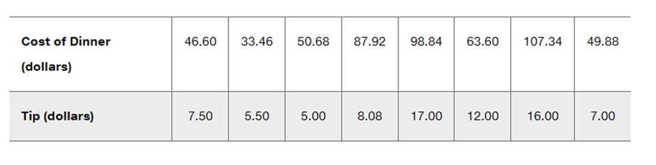
Problem 10.CQQ.1

Exercises 1–10 are based on the following sample data consisting of costs of dinner (dollars) and the amounts of tips (dollars) left by diners. The data were collected by students of the author.

[IMAGE]

Scatterplot Construct a scatterplot and comment on the pattern of points.

Problem 10.CQQ.6

Exercises 1–10 are based on the following sample data consisting of costs of dinner (dollars) and the amounts of tips (dollars) left by diners. The data were collected by students of the author.

[IMAGE]

Change in Scale Exercise 1 stated that for the given paired data, r = 0.846. How does that value change if all of the amounts of dinners are left unchanged but all of the tips are expressed in cents instead of dollars?

Problem 10.CQQ.8

Exercises 1–10 are based on the following sample data consisting of costs of dinner (dollars) and the amounts of tips (dollars) left by diners. The data were collected by students of the author.

Predictions The sample data result in a linear correlation coefficient of r = 0.846 and the regression equation y^ = -0.00777 + 0.145x. What is the best predicted amount of tip, given that the cost of dinner was $84.62? How was the predicted value found?

Problem 10.CQQ.3

Exercises 1–10 are based on the following sample data consisting of costs of dinner (dollars) and the amounts of tips (dollars) left by diners. The data were collected by students of the author.

[IMAGE]

Fixed Percentage If a restaurant were to change its tipping policy so that a constant tip of 20% of the bill is added to the cost of the dinner, what would be the value of the linear correlation coefficient for the paired amounts of dinners/tips?

Problem 10.RE.3c

Time and Motion In a physics experiment at Doane College, a soccer ball was thrown upward from the bed of a moving truck. The table below lists the time (sec) that has lapsed from the throw and the corresponding height (m) of the soccer ball.

[IMAGE]

c. What horrible mistake would be easy to make if the analysis is conducted without a scatterplot?

Problem 10.RE.3a

[IMAGE]

a. Find the value of the linear correlation coefficient r.