Triola - Elementary Statistics 14th Edition

Ch. 10 - Correlation and Regression

Back

All textbooks

Triola 14th Edition

Ch. 10 - Correlation and Regression

Problem 10.2.4

Correlation and Slope What is the relationship between the linear correlation coefficient r and the slope b1 of a regression line?

Problem 10.1.16

Testing for a Linear Correlation

In Exercises 13–28, construct a scatterplot, and find the value of the linear correlation coefficient r. Also find the P-value or the critical values of r from Table A-6. Use a significance level of α = 0.05. Determine whether there is sufficient evidence to support a claim of a linear correlation between the two variables. (Save your work because the same data sets will be used in Section 10-2 exercises.)

Taxis Using the data from Exercise 15, is there sufficient evidence to support the claim that there is a linear correlation between the distance of the ride and the tip amount? Does it appear that riders base their tips on the distance of the ride?

Problem 10.5.11

Finding the Best Model

In Exercises 5–16, construct a scatterplot and identify the mathematical model that best fits the given data. Assume that the model is to be used only for the scope of the given data, and consider only linear, quadratic, logarithmic, exponential, and power models.

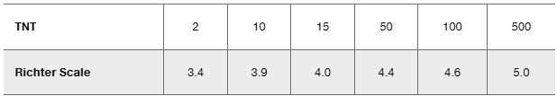
Richter Scale The table lists different amounts (metric tons) of the explosive TNT and the corresponding value measured on the Richter scale resulting from explosions of the TNT.

Problem 10.2.29

Large Data Sets

Exercises 29–32 use the same Appendix B data sets as Exercises 29–32 in Section 10-1. In each case, find the regression equation, letting the first variable be the predictor (x) variable. Find the indicated predicted values following the prediction procedure summarized in Figure 10-5.

Taxis Repeat Exercise 15 using all of the time/tip data from the 703 taxi rides listed in Data Set 32 “Taxis” from Appendix B.

Problem 10.2.30

Large Data Sets

Taxis Repeat Exercise 16 using all of the distance/tip data from the 703 taxi rides listed in Data Set 32 “Taxis” from Appendix B.

Problem 10.5.17

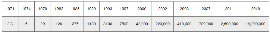
Moore’s Law In 1965, Intel cofounder Gordon Moore initiated what has since become known as Moore’s law: The number of transistors per square inch on integrated circuits will double approximately every 18 months. In the table below, the first row lists different years and the second row lists the number of transistors (in thousands) for different years.

Ignoring the listed data and assuming that Moore’s law is correct and transistors per square inch double every 18 months, which mathematical model best describes this law: linear, quadratic, logarithmic, exponential, power? What specific function describes Moore’s law?

Which mathematical model best fits the listed sample data?

Compare the results from parts (a) and (b). Does Moore’s law appear to be working reasonably well?

Problem 10.5.5

Finding the Best Model

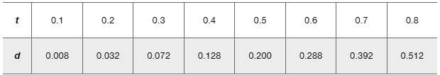
Landing on the Moon When the Apollo spacecraft landed on the Moon, the rocket engine would typically cut off at about 1.3 meters above the surface so that hot gases and dust and other surface materials would not cause damage. The landing module was in freefall starting at about 1 meter above the surface. The table below lists the time t (seconds) after being dropped and the distance d (meters) travelled by an object dropped near the surface of the Moon.

Problem 10.4.19

Dummy Variable Refer to Data Set 18 “Bear Measurements” in Appendix B and use the sex, age, and weight of the bears. For sex, let 0 represent female and let 1 represent male. Letting the response variable represent weight, use the variable of age and the dummy variable of sex to find the multiple regression equation. Use the equation to find the predicted weight of a bear with the characteristics given below. Does sex appear to have much of an effect on the weight of a bear?

Female bear that is 20 years of age

Male bear that is 20 years of age

Problem 10.4.7

Interpreting a Computer Display

In Exercises 5–8, we want to consider the correlation between heights of fathers and mothers and the heights of their sons. Refer to the StatCrunch display and answer the given questions or identify the indicated items. The display is based on Data Set 10 “Family Heights” in Appendix B. (The response y variable represents heights of sons.)

[IMAGE]

Height of Son Should the multiple regression equation be used for predicting the height of a son based on the height of his father and mother? Why or why not?

Problem 10.2.9

Finding the Equation of the Regression Line

In Exercises 9 and 10, use the given data to find the equation of the regression line. Examine the scatterplot and identify a characteristic of the data that is ignored by the regression line.

[IMAGE]

Problem 10.2.19

Regression and Predictions

Exercises 13–28 use the same data sets as Exercises 13–28 in Section 10-1.

Find the regression equation, letting the first variable be the predictor (x) variable.

Find the indicated predicted value by following the prediction procedure summarized in Figure 10-5.

Oscars Listed below are ages of recent Oscar winners matched by the years in which the awards were won (from Data Set 21 “Oscar Winner Age” in Appendix B). Find the best predicted age of an Oscar-winning actress given that the Oscar winner for best actor is 59 years of age. How does the result compare to the actual actress age of 60 years?

[IMAGE]

Problem 10.1.2

Notation The author conducted an experiment in which the height of each student was measured in centimeters and those heights were matched with the same students’ scores on the first statistics test. If we find that r = 0, does that indicate that there is no association between those two variables?

Problem 10.5.7

Finding the Best Model

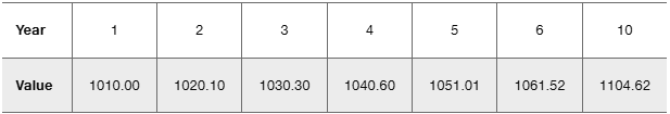
CD Yields The table lists the value y (in dollars) of $1000 deposited in a certificate of deposit at Bank of New York (based on rates currently in effect).

Problem 10.4.1

Response and Predictor Variables Using all of the Tour de France bicycle race results up to a recent year, we get this multiple regression equation: Speed = 29.2-0.00260Distance + 0.540Stages + 0.0570Finishers, where Speed is the mean speed of the winner (km/h), Distance is the length of the race (km), Stages is the number of stages in the race, and Finishers is the number of bicyclists who finished the race. Identify the response and predictor variables.

Problem 10.2.6

Making Predictions

In Exercises 5–8, let the predictor variable x be the first variable given. Use the given data to find the regression equation and the best predicted value of the response variable. Be sure to follow the prediction procedure summarized in Figure 10-5. Use a 0.05 significance level.

Bear Measurements Head widths (in.) and weights (lb) were measured for 20 randomly selected bears (from Data Set 18 “Bear Measurements” in Appendix B). The 20 pairs of measurements yield xbar = 6.9 in., ybar = 214.3 lb, r = 0.879 P-value = 0.000 and y^ = -212 + 61.9x. Find the best predicted weight of a bear given that the bear has a head width of 6.5 in.

Problem 10.2.14

Regression and Predictions

Exercises 13–28 use the same data sets as Exercises 13–28 in Section 10-1.

Find the regression equation, letting the first variable be the predictor (x) variable.

Find the indicated predicted value by following the prediction procedure summarized in Figure 10-5.

Powerball Jackpots and Tickets Sold Listed below are the same data from Table 10-1 in the Chapter Problem, but an additional pair of values has been added from actual Powerball results. (Jackpot amounts are in millions of dollars, ticket sales are in millions.) Find the best predicted number of tickets sold when the jackpot was actually 345 million dollars. How does the result compare to the value of 55 million tickets that were actually sold?

Problem 10.5.16

Finding the Best Model

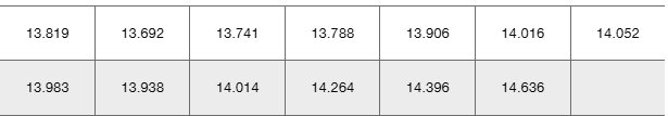
Global Warming Listed below are mean annual temperatures (°C) of the earth for each decade, beginning with the decade of the 1880s. Find the best model and then predict the value for 2090–2099. Comment on the result.

Problem 10.2.22

Regression and Predictions

Exercises 13–28 use the same data sets as Exercises 13–28 in Section 10-1.

Find the regression equation, letting the first variable be the predictor (x) variable.

Find the indicated predicted value by following the prediction procedure summarized in Figure 10-5.

Subway and the CPI Use the subway/CPI data from the preceding exercise. What is the best predicted value of the CPI when the subway fare is $3.00?

Problem 10.5.12

Finding the Best Model

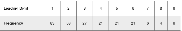
Detecting Fraud Leading digits of check amounts are often analyzed for the purpose of detecting fraud. The accompanying table lists frequencies of leading digits from checks written by the author (an honest guy).

Problem 10.1.15

Testing for a Linear Correlation

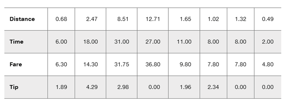
Taxis The table below includes data from New York City taxi rides (from Data Set 32 “Taxis” in Appendix B). The distances are in miles, the times are in minutes, the fares are in dollars, and the tips are in dollars. Is there sufficient evidence to support the claim that there is a linear correlation between the time of the ride and the tip amount? Does it appear that riders base their tips on the time of the ride?

Problem 10.3.20

Variation and Prediction Intervals

In Exercises 17–20, find the (a) explained variation, (b) unexplained variation, and (c) indicated prediction interval. In each case, there is sufficient evidence to support a claim of a linear correlation, so it is reasonable to use the regression equation when making predictions.

Weighing Seals with a Camera The table below lists overhead widths (cm) of seals measured from photographs and the weights (kg) of the seals (based on “Mass Estimation of Weddell Seals Using Techniques of Photogrammetry,” by R. Garrott of Montana State University). For the prediction interval, use a 99% confidence level with an overhead width of 9.0 cm.

Problem 10.5.13

Finding the Best Model

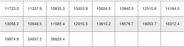
Stock Market Listed below in order by row are the annual high values of the Dow Jones Industrial Average for each year beginning with 2000. Find the best model and then predict the value for the last year listed. Is the predicted value close to the actual value of 26,828.4?

Problem 10.2.2

Notation What is the difference between the regression equation y^ = b0 + b1x and the regression equation y = β0 + β1x.

Problem 10.3.5

Interpreting the Coefficient of Determination

In Exercises 5–8, use the value of the linear correlation coefficient r to find the coefficient of determination and the percentage of the total variation that can be explained by the linear relationship between the two variables.

Times of Taxi Rides and Tips r = 0.298 (x = time in minutes, y = the amount of tip in dollars)

Problem 10.5.6

Finding the Best Model

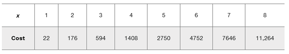
Dirt Cheap The Cherry Hill Construction company in Branford, CT sells screened topsoil by the “yard,” which is actually a cubic yard. Let the variable x be the length (yd) of each side of a cube of screened topsoil. The table below lists the values of x along with the corresponding cost (dollars).

Problem 10.5.4

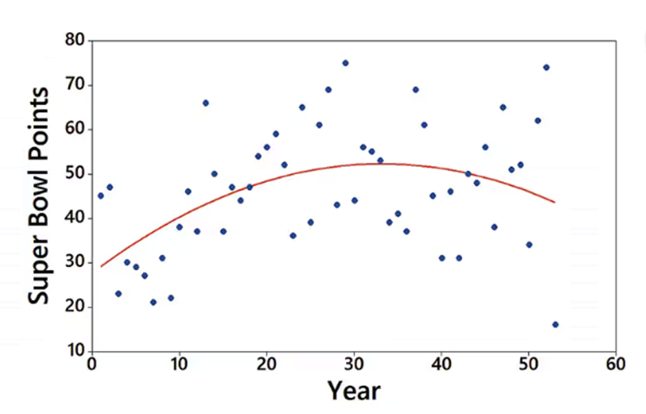
Interpreting a Graph The accompanying graph plots the numbers of points scored in each Super Bowl from the first Super Bowl in 1967 (coded as year 1) to the last Super Bowl at the time of this writing. The graph of the quadratic equation that best fits the data is also shown in red. What feature of the graph justifies the value of R^2 = 0.205 for the quadratic model?

Problem 10.5.14

Finding the Best Model

Sunspot Numbers Listed below in order by row are annual sunspot numbers beginning with 1980. Is the best model a good model? Carefully examine the scatterplot and identify the pattern of the points. Which of the models fits that pattern?

[IMAGE]

Problem 10.3.8

Interpreting the Coefficient of Determination

Times of Taxi Rides and Fares r = 0.953 (x = time in minutes, y = fare in dollars)

Problem 10.5.2

Super Bowl and R^2 Let x represent years coded as 1,1,3,... for years starting in 1980, and let y represent the numbers of points scored in each annual Super Bowl beginning in 1980. Using the data from 1980 to the last Super Bowl at the time of this writing, we obtain the following values of R^2 for the different models: linear: 0.008; quadratic: 0.023; logarithmic: 0.0004; exponential: 0.027; power: 0.007. Based on these results, which model is best? Is the best model a good model? What do the results suggest about predicting the number of points scored in a future Super Bowl game?

Problem 10.1.14

Testing for a Linear Correlation

Powerball Jackpots and Tickets Sold Listed below are the same data from Table 10-1 in the Chapter Problem, but an additional pair of values has been added from actual Powerball results. Is there sufficient evidence to conclude that there is a linear correlation between lottery jackpots and numbers of tickets sold? Comment on the effect of the added pair of values in the last column. Compare the results to those obtained in Example 4.