Discrete random variables are characterized by a finite set of values they can take, such as the outcomes of rolling a die. These values can be represented in a table or graph, where the x-axis displays the possible values and the height of the bars indicates their probabilities. Notably, there are gaps between the bars, reflecting that certain values cannot occur simultaneously, such as being greater than one and less than two.
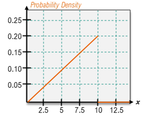
In contrast, continuous random variables can take on any value within a specified range, making them infinitely divisible. For instance, if a continuous random variable x can range from 0 to 6, it can assume any value within that interval, including decimals and irrational numbers like π. This characteristic necessitates the use of a probability density function (PDF) to represent continuous random variables, as listing all possible values in a table is impractical.
To find probabilities for discrete random variables, one can sum the probabilities of the individual values within a specified range. For example, to determine the probability that x is between 1 and 3, one would identify the values (1, 2, and 3) and their associated probabilities, which might each be 1/6, leading to a total probability of 1/2.
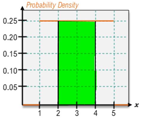
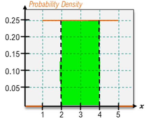
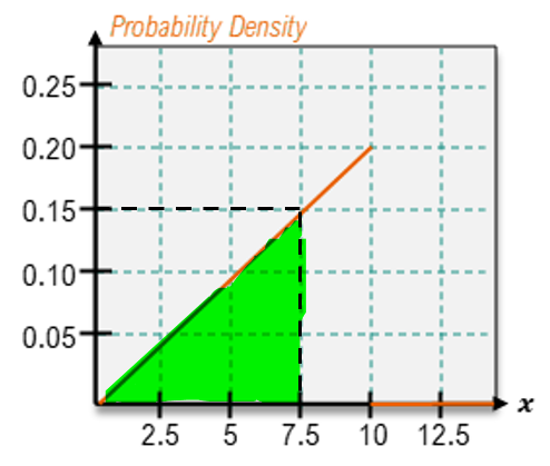
For continuous random variables, however, the approach differs significantly. Instead of summing probabilities, one calculates the area under the PDF over the desired range. For example, to find the probability that x is between 1 and 3, one would calculate the area of the rectangle formed by the PDF between these two points. If the height of the rectangle is determined to be 1/6 and the width is 2 (from 1 to 3), the area—and thus the probability—would be (1/6) * 2 = 2/6 or 1/3.
When considering the probability of x taking on a specific value, such as 5, the discrete case allows for a straightforward lookup in the probability table, yielding a probability of 1/6. In contrast, for continuous random variables, the probability of x being exactly 5 is zero. This is because, while 5 is a possible value, there are infinitely many other values within the range, making the probability of selecting any single value effectively zero. This concept can be understood as the probability of a single point in a continuous distribution being 1 divided by infinity, which approaches zero.
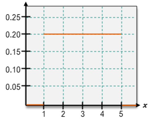
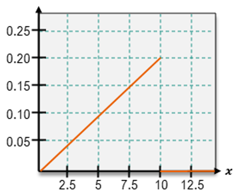
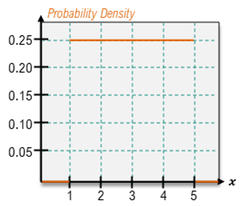
One important type of continuous distribution is the uniform distribution, where the PDF maintains a constant height across all values of x. This means that every value within the range has the same probability density. The uniform distribution is a specific case of continuous random variables, and not all continuous distributions exhibit this property. To identify a uniform distribution, one can check if the height of the PDF remains consistent for all possible values of x.
Understanding these distinctions between discrete and continuous random variables, as well as the methods for calculating their probabilities, is crucial for effectively analyzing and interpreting data in various fields.
 ;
;  ;
;  ;
;  ;
; 
 ;
;  ;
;  ;
;