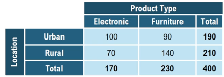
Understanding the relationship between two variables can provide valuable insights, especially in educational contexts. For instance, when examining students' heights in relation to their grade levels, a contingency table becomes an essential tool. A contingency table is a type of frequency distribution that displays the frequencies of different categories across two variables, allowing for a clearer analysis of their relationship.
To illustrate, consider a scenario involving the heights and grade levels of 161 students in ninth and tenth grades. By organizing this data into a contingency table, one can easily determine how many students fall into specific height ranges within each grade. For example, to find the number of ninth graders whose heights range from 5'1" to 5'6", one would look at the intersection of the corresponding row and column in the table, revealing an observed frequency of 40 students.
In cases where the inquiry involves a broader range, such as the total number of students between 6'1" and 6'6", it is necessary to sum the observed frequencies from both grade levels. This approach highlights the importance of understanding how to navigate the table effectively, as it allows for quick calculations and insights.
Moving beyond observed frequencies, expected frequencies provide a theoretical framework for understanding what one might anticipate if the two variables were independent. The expected frequency for a specific cell in the table can be calculated using the formula:
E = \frac{(Row \ Total) \times (Column \ Total)}{Grand \ Total}
Here, the row total represents the number of students in a specific category (e.g., ninth graders), while the column total reflects the number of students within a particular height range. The grand total is the overall number of students surveyed. For instance, if there are 77 ninth graders and 72 students between 5'1" and 5'6", the expected frequency for that cell would be calculated as:
E = \frac{77 \times 72}{161} \approx 34.43
This indicates that, under the assumption of independence, one would expect approximately 34.43 ninth graders to fall within that height range, contrasting with the observed frequency of 40.
Calculating expected frequencies for other cells follows the same principle, adjusting the column total as necessary. For example, if the column total changes to 61 for a different height range, the expected frequency would be:
E = \frac{77 \times 61}{161} \approx 29.17
By systematically applying this method across all cells in the contingency table, one can derive a comprehensive understanding of the data, facilitating further analysis and interpretation. This approach not only enhances data literacy but also equips students with the skills to analyze relationships between multiple variables effectively.


