Introduction to Contingency Tables: Videos & Practice Problems

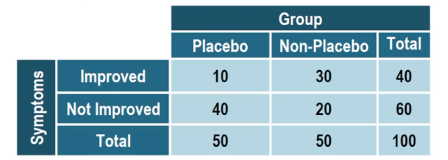
When analyzing data involving two categorical variables, contingency tables serve as a valuable tool to display frequencies. These tables allow us to explore relationships between variables, such as whether a student drives a car and their grade level. Each cell in the table represents the frequency of responses that fit both categories, making it easy to visualize the data.

To interpret a contingency table, identify the row and column corresponding to the variables of interest. For instance, if a cell shows the number 30 in the junior row and the no column, it indicates that 30 juniors do not drive a car. Additionally, contingency tables often include total rows and columns, which summarize the counts for each category, helping to understand the overall distribution of responses.

Understanding probabilities within this context involves three key types: marginal, joint, and conditional probabilities. Marginal probability refers to the likelihood of a single category occurring, calculated by dividing the total of that category by the grand total. For example, if 60 out of 100 students drive a car, the marginal probability of driving a car is:

$$ P(\text{drives a car}) = \frac{60}{100} = 0.6 $$

Joint probability, on the other hand, assesses the likelihood of two events occurring simultaneously. This is determined by taking the frequency from the relevant cell and dividing it by the grand total. For instance, if 40 seniors drive a car, the joint probability is:

$$ P(\text{senior and drives a car}) = \frac{40}{100} = 0.4 $$

Conditional probability evaluates the likelihood of one event occurring given that another event has already happened. This is calculated by taking the frequency from the relevant cell and dividing it by the total of the row or column that corresponds to the known event. For example, to find the probability that a student drives a car given they are a senior, you would use the frequency of seniors who drive a car (40) and divide it by the total number of seniors (50):

$$ P(\text{drives a car | senior}) = \frac{40}{50} = 0.8 $$

Recognizing the differences between these probabilities is crucial for accurately interpreting data. Marginal probability focuses on one category, joint probability looks at the intersection of two events, and conditional probability considers the likelihood of an event based on a known condition. Mastering these concepts will enhance your ability to analyze and draw conclusions from categorical data effectively.

In this exercise, we will construct a contingency table based on survey data regarding hair and eye color among 50 individuals. The grand total of surveyed individuals is 50, which will be reflected in both the total column and total row of the table.

First, we note that 28% of the surveyed individuals have blue eyes. Calculating this, we find that 28% of 50 equals 14, indicating that 14 people have blue eyes. This value is placed in the total row of the blue-eyed column.

Similarly, we are informed that 28% of the individuals are blonde, which also results in 14 people. This number is recorded in the total column of the blonde-haired row.

Next, we learn that 20% of the surveyed individuals are both blonde and blue-eyed. Calculating 20% of 50 gives us 10, which we place in the cell where the blonde hair and blue eyes intersect.

It is also stated that no individuals have both black hair and hazel eyes, so we enter a zero in the corresponding cell for this combination.

Continuing, we find that 40% of the individuals have brown hair. This translates to 20 people, which we place in the total cell of the brown-haired row. Since we have accounted for 34 individuals with either brown or blonde hair, the remaining individuals must have black hair, totaling 16.

Next, we are told that 60% of the individuals have brown eyes, which amounts to 30 people. This value is recorded in the total row of the brown-eyed column. By subtracting the accounted individuals, we determine that 6 individuals must have hazel eyes.

We also learn that one out of seven blue-eyed individuals has black hair. With 14 blue-eyed individuals, this means there are 2 individuals with both blue eyes and black hair, which we place in the corresponding cell.

From the previous calculations, we know that among the 14 blue-eyed individuals, 10 have blonde hair, leaving 2 who must have brown hair. Additionally, we find that 50% of the 6 individuals with hazel eyes have blonde hair, resulting in 3 individuals. The remaining 3 hazel-eyed individuals must have brown hair.

To complete the table, we can fill in the remaining cells using the totals. For instance, since 14 individuals have blonde hair and we have accounted for 13 of them with blue or hazel eyes, the remaining individual must have brown eyes. For the 20 individuals with brown hair, we have accounted for 5 with hazel or blue eyes, leaving 15 who must have brown eyes. Finally, for the 16 individuals with black hair, we have accounted for 2 with blue eyes and none with hazel eyes, meaning the remaining 14 must have brown eyes.

This structured approach allows us to visualize the relationships between hair and eye color effectively, providing a clear overview of the surveyed population.

In this analysis, we explore the dietary preferences of wedding guests through the lens of conditional and marginal distributions. Conditional distribution focuses on the probabilities of certain characteristics given a specific condition, while marginal distribution provides an overview of the overall distribution of categories within a dataset.

To determine the conditional distribution for vegetarians, we first calculate the probability of guests having allergies based on their vegetarian status. Out of 13 vegetarians, 9 do not have allergies. Thus, the probability of no allergies given that a guest is vegetarian is:

$$ P(\text{No Allergies} | \text{Vegetarian}) = \frac{9}{13} \approx 0.69 \text{ or } 69\% $$

Conversely, the probability of having allergies given that a guest is vegetarian is calculated as follows. Among the 13 vegetarians, 4 have allergies, leading to:

$$ P(\text{Allergies} | \text{Vegetarian}) = \frac{4}{13} \approx 0.31 \text{ or } 31\% $$

This indicates that approximately 69% of vegetarians do not have allergies, while 31% do.

Next, we turn our attention to the marginal distribution of diet types, which summarizes the overall percentages of each dietary category among all guests. With a total of 85 guests, we find the following probabilities:

1. The probability of a guest being vegetarian is:

$$ P(\text{Vegetarian}) = \frac{13}{85} \approx 0.15 \text{ or } 15\% $$

2. The probability of a guest being vegan is:

$$ P(\text{Vegan}) = \frac{7}{85} \approx 0.08 \text{ or } 8\% $$

3. The probability of a guest being neither vegetarian nor vegan is:

$$ P(\text{Neither}) = \frac{65}{85} \approx 0.76 \text{ or } 76\% $$

While the percentages do not sum to exactly 100% due to rounding, the results clearly show that approximately 15% of the guests are vegetarian, 8% are vegan, and 76% are neither. This analysis provides valuable insights into the dietary preferences of the wedding guests, highlighting the importance of understanding conditional and marginal distributions in data interpretation.