Using and Interpreting Concepts

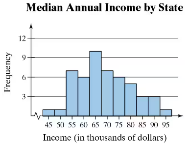
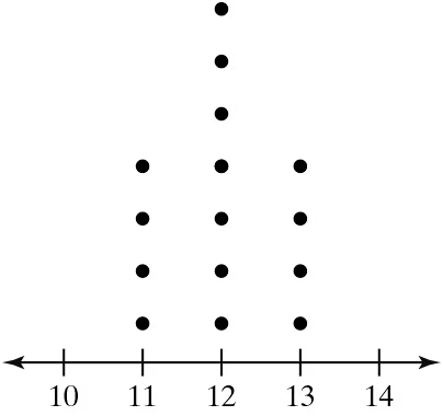
Finding the Range of a Data Set In Exercises 9 and 10, find the range of the data set represented by the graph.

Archaeology The depths (in inches) at which 10 artifacts are found are listed. 

20.7 24.8 30.5 26.2 36.0 34.3 30.3 29.5 27.0 38.5

a. Find the range of the data set.

In Exercises 13 and 14, find the range, mean, variance, and standard deviation of the population data set.

Drunk Driving The number of alcohol-impaired crash fatalities (in thousands) per year from 2010 through 2019 (Source: National Highway Traffic Safety Administration)

10.1 9.9 10.3 10.1 9.9 10.3 11.0 10.9 10.7 10.1

Finding Sample Statistics In Exercises 15 and 16, find the range, mean, variance, and standard deviation of the sample data set.

Pregnancy Durations The durations (in days) of pregnancies for a random sample of pregnant people

277 291 295 280 268 278 291

277 282 279 296 285 269 293

267 281 286 269 264 299 275

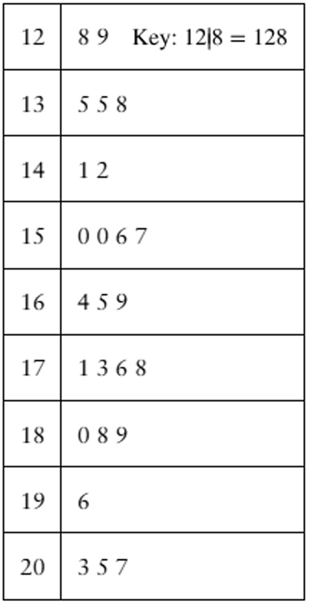
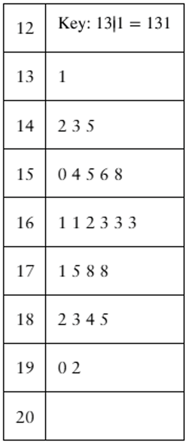
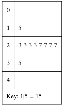
Estimating Standard Deviation Both data sets shown in the stem-and-leaf plots have a mean of 165. One has a standard deviation of 16, and the other has a standard deviation of 24. By looking at the stem-and-leaf plots, which is which? Explain your reasoning.

Salary Offers You are applying for jobs at two companies. Company C offers starting salaries with μ = $59,000 and σ = $1500. Company D offers starting salaries with μ = $59,000 and σ = $1000. From which company are you more likely to get an offer of $62,000 or more? Explain your reasoning.

Estimating the Sample Mean and Standard Deviation for Grouped Data In Exercises 41–44, make a frequency distribution for the data. Then use the table to estimate the sample mean and the sample standard deviation of the data set.

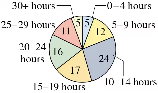
Weekly Study Hours The distribution of the number of hours that a random sample of college students study per week is shown in the pie chart. Use 32 as the midpoint for “30+ hours.”

Using Chebychev’s Theorem Old Faithful is a famous geyser at Yellowstone National Park. From a sample with n = 100, the mean interval between Old Faithful’s eruptions is 101.56 minutes and the standard deviation is 42.69 minutes. Using Chebychev’s Theorem, determine at least how many of the intervals lasted between 16.18 minutes and 186.94 minutes. (Adapted from Geyser Times)

Finding the Sample Mean and Standard Deviation for Grouped Data In Exercises 39 and 40, make a frequency distribution for the data. Then use the table to find the sample mean and the sample standard deviation of the data set.

3 3 5 3 8 0 3 9 6 6 7 1 6 3 2 6 9 1 8 5 0 2 3 4 9

5 8 1 9 7 6 9 6 7 0 6 3 8 6 8 7 3 8 9 3 7 2 4 4 1

Constructing Data Sets In Exercises 25–28, construct a data set that has the given statistics.

N = 6

μ = 5

σ ≈ 2

Constructing Data Sets In Exercises 25–28, construct a data set that has the given statistics.

n = 6

x̄ = 7

s ≈ 2

Using the Empirical Rule In Exercises 29–34, use the Empirical Rule.

Use the sample statistics from Exercise 29 and assume the number of vehicles in the sample is 75.

a. Estimate the number of vehicles whose speeds are between 63 miles per hour and 71 miles per hour.

Using the Empirical Rule In Exercises 29–34, use the Empirical Rule.

The speeds for eight vehicles are listed. Using the sample statistics from Exercise 29, determine which of the data entries are unusual. Are any of the data entries very unusual? Explain your reasoning.

70, 78, 62, 71, 65, 76, 82, 64

Shifting Data Sample annual salaries (in thousands of dollars) for employees at a company are listed.

40   35   49   53   38   39   40

37   49   34   38   43   47   35

c. Each employee in the sample takes a pay cut of $2000 from their original salary. Find the sample mean and the sample standard deviation for the revised data set.

Mean Absolute Deviation Another useful measure of variation for a data set is the mean absolute deviation (MAD). It is calculated by the formula

MAD = Σ |x − x̄| / n.

b. Find the mean absolute deviation of the data set in Exercise 16. Compare your result with the sample standard deviation obtained in Exercise 16.

Scaling Data Sample annual salaries (in thousands of dollars) for employees at a company are listed.

42   36   48   51   39   39   42

36   48   33   39   42   45   50

b. Each employee in the sample receives a 5% raise. Find the sample mean and the sample standard deviation for the revised data set.

Extending Concepts

Alternative Formula You used SSₓ = Σ(x − x̄)² when calculating variance and standard deviation. An alternative formula that is sometimes more convenient for hand calculations is

SSₓ = Σ x² − (Σ x)² / n.

You can find the sample variance by dividing the sum of squares by n − 1 and the sample standard deviation by finding the square root of the sample variance.

b. Use the alternative formula to calculate the sample standard deviation for the data set in Exercise 15.

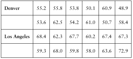
Comparing Variation in Different Data Sets In Exercises 45–50, find the coefficient of variation for each of the two data sets. Then compare the results.

Annual Salaries Sample annual salaries (in thousands of dollars) for entry level architects in Denver, CO, and Los Angeles, CA, are listed.

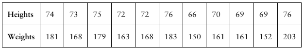
Comparing Variation in Different Data Sets In Exercises 45–50, find the coefficient of variation for each of the two data sets. Then compare the results.

Heights and Weights The heights (in inches) and weights (in pounds) of every France national soccer team player that started the 2018 FIFA Men’s World Cup final are listed. (Source: ESPN)

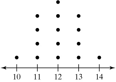
Graphical Analysis In Exercises 21–24, you are asked to compare three data sets.

(c) Estimate the sample standard deviations. Then determine how close each of your estimates is by finding the sample standard deviations.

i.

ii.

iii.

Pearson’s Index of Skewness The English statistician Karl Pearson (1857–1936) introduced a formula for the skewness of a distribution.

P = 3 (x̄ - median) / s

Most distributions have an index of skewness between -3 and 3. When P > 0, the data are skewed right. When P < 0, the data are skewed left. When P = 0, the data are symmetric. Calculate the coefficient of skewness for each distribution. Describe the shape of each.

a. x̄ = 17, s = 2.3, median = 19

Pearson’s Index of Skewness The English statistician Karl Pearson (1857–1936) introduced a formula for the skewness of a distribution.

P = 3 (x̄ - median) / s

Most distributions have an index of skewness between -3 and 3. When P > 0, the data are skewed right. When P < 0, the data are skewed left. When P = 0, the data are symmetric. Calculate the coefficient of skewness for each distribution. Describe the shape of each.

c. x̄ = 9.2, s = 1.8, median = 9.2

Pearson’s Index of Skewness The English statistician Karl Pearson (1857–1936) introduced a formula for the skewness of a distribution.

P = 3 (x̄ - median) / s

Most distributions have an index of skewness between -3 and 3. When P > 0, the data are skewed right. When P < 0, the data are skewed left. When P = 0, the data are symmetric. Calculate the coefficient of skewness for each distribution. Describe the shape of each.

e. x̄ = 155, s = 20.0, median = 175

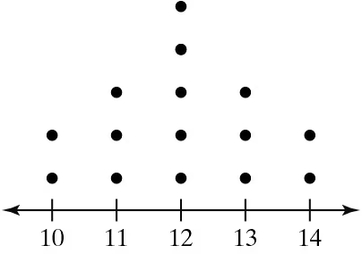
Graphical Analysis In Exercises 21–24, you are asked to compare three data sets.

(c) Estimate the sample standard deviations. Then determine how close each of your estimates is by finding the sample standard deviations.

i. ii. iii.

Building Basic Skills and Vocabulary

The length of a guest lecturer’s talk represents the third quartile for talks in a guest lecture series. Make an observation about the length of the talk.

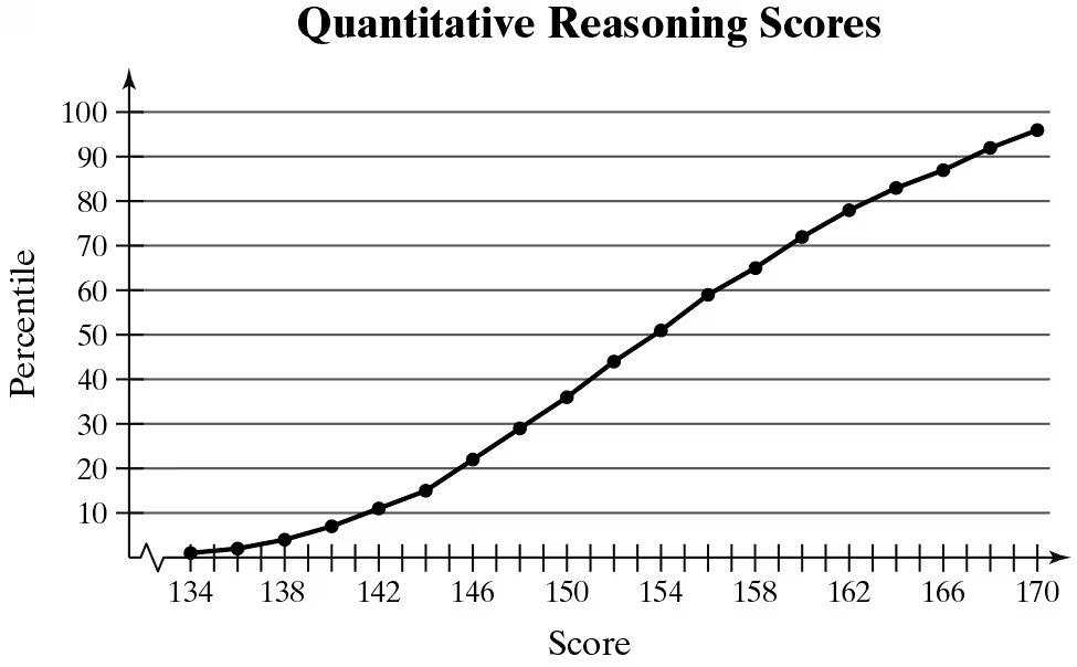
Interpreting Percentiles In Exercises 29–32, use the ogive, which represents the cumulative frequency distribution for quantitative reasoning scores on the Graduate Record Examination in a recent range of years. (Adapted from Educational Testing Service)

What percentile is a score of 170? How should you interpret this?

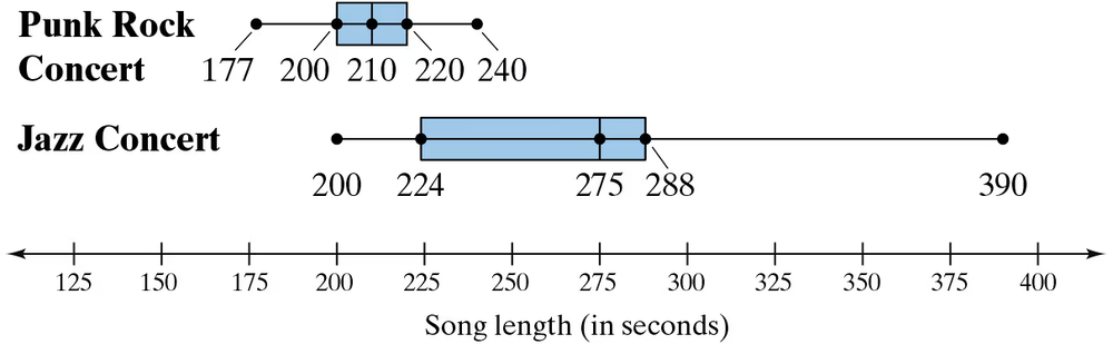
Song Lengths Side-by-side box-and-whisker plots can be used to compare two or more different data sets. Each box-and-whisker plot is drawn on the same number line to compare the data sets more easily. The lengths (in seconds) of songs played at two different concerts are shown.

a. Describe the shape of each distribution. Which concert has less variation in song lengths?

Song Lengths Side-by-side box-and-whisker plots can be used to compare two or more different data sets. Each box-and-whisker plot is drawn on the same number line to compare the data sets more easily. The lengths (in seconds) of songs played at two different concerts are shown.

d. Can you determine which concert lasted longer? Explain.

Modified Box-and-Whisker Plot In Exercises 59–62, (a) identify any outliers and (b) draw a modified box-and-whisker plot that represents the data set. Use asterisks (*) to identify outliers.

75 78 80 75 62 72 74 75 80 95 76 72

Drawing a Box-and-Whisker Plot In Exercises 15–18,

(b) draw a box-and-whisker plot that represents the data set.

39 36 30 27 26 24 28 35 39 60 50 41 35 32 51