Back
BackProblem 2.1.45b
What Would You Do? You work at a bank and are asked to recommend the amount of cash to put in an ATM each day. You do not want to put in too much (which would cause security concerns) or too little (which may create customer irritation). The daily withdrawals (in hundreds of dollars) for 30 days are listed. 72 84 61 76 104 76 86 92 80 88 98 76 97 82 84 67 70 81 82 89 74 73 86 81 85 78 82 80 91 83
If you put $9000 in the ATM each day, what percent of the days in a month should you expect to run out of cash? Explain.
Problem 2.5.28b
Hourly Earnings Refer to the data set in Exercise 26 and the box-and-whisker plot you drew that represents the data set.
b. What percent of the employees made more than $23.39 per hour?
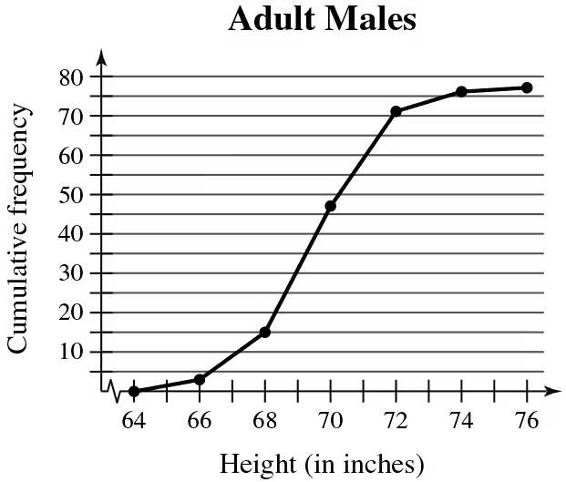
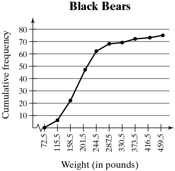
Problem 2.1.28b
Use the ogive to approximate
the height for which the cumulative frequency is 15.
Problem 2.3.66b
Extending Concepts
Trimmed Mean To find the 10% trimmed mean of a data set, order the data, delete the lowest 10% of the entries and the highest 10% of the entries, and find the mean of the remaining entries.
b. Compare the four measures of central tendency, including the midrange.
Problem 2.5.11b
Using and Interpreting Concepts
Using and Interpreting Concepts Finding Quartiles, Interquartile Range, and Outliers In Exercises 11 and 12,
(b) find the interquartile range
56 63 51 60 57 60 60 54 63 59 80 63 60 62 65
Problem 2.4.52b
Mean Absolute Deviation Another useful measure of variation for a data set is the mean absolute deviation (MAD). It is calculated by the formula
MAD = Σ |x − x̄| / n.
b. Find the mean absolute deviation of the data set in Exercise 16. Compare your result with the sample standard deviation obtained in Exercise 16.
Problem 2.5.49b
Life Spans of Tires A brand of automobile tire has a mean life span of 35,000 miles, with a standard deviation of 2250 miles. Assume the life spans of the tires have a bell-shaped distribution.
b. The life spans of three randomly selected tires are 30,500 miles, 37,250 miles, and 35,000 miles. Using the Empirical Rule, find the percentile that corresponds to each life span.
Problem 2.4.54c
Shifting Data Sample annual salaries (in thousands of dollars) for employees at a company are listed.
40 35 49 53 38 39 40
37 49 34 38 43 47 35
c. Each employee in the sample takes a pay cut of $2000 from their original salary. Find the sample mean and the sample standard deviation for the revised data set.
Problem 2.3.62c
Extending Concepts
Golf The distances (in yards) for nine holes of a golf course are listed.
336 393 408 522 147 504 177 375 360
c. Compare the measures you found in part (b) with those found in part (a). What do you notice?
Problem 2.4.22c
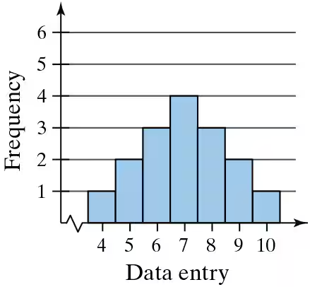
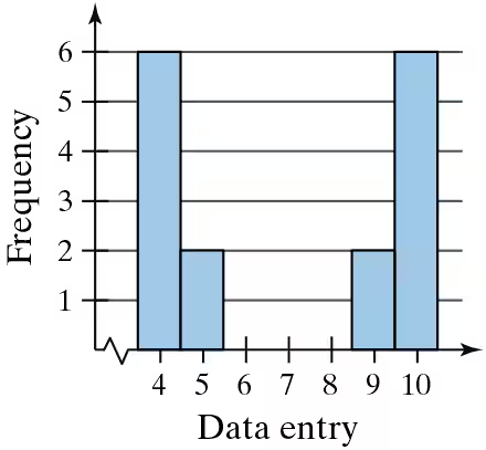
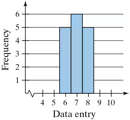
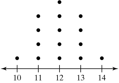
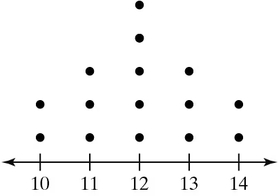
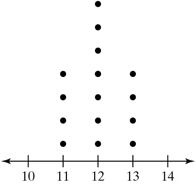
Graphical Analysis In Exercises 21–24, you are asked to compare three data sets.
(c) Estimate the sample standard deviations. Then determine how close each of your estimates is by finding the sample standard deviations.
i.
ii.
iii.
Problem 2.1.43c
Use the data set and the indicated number of classes to construct
(c) a frequency polygon,
Pulse Rates
Number of classes: 6 Data set: Pulse rates of all students in a class 68 105 95 80 90 100 75 70 84 98 102 70 65 88 90 75 78 94 110 120 95 80 76 108
Problem 2.3.66c
Extending Concepts
Trimmed Mean To find the 10% trimmed mean of a data set, order the data, delete the lowest 10% of the entries and the highest 10% of the entries, and find the mean of the remaining entries.
c. What is the benefit of using a trimmed mean versus using a mean found using all data entries? Explain your reasoning.
Problem 2.1.24c
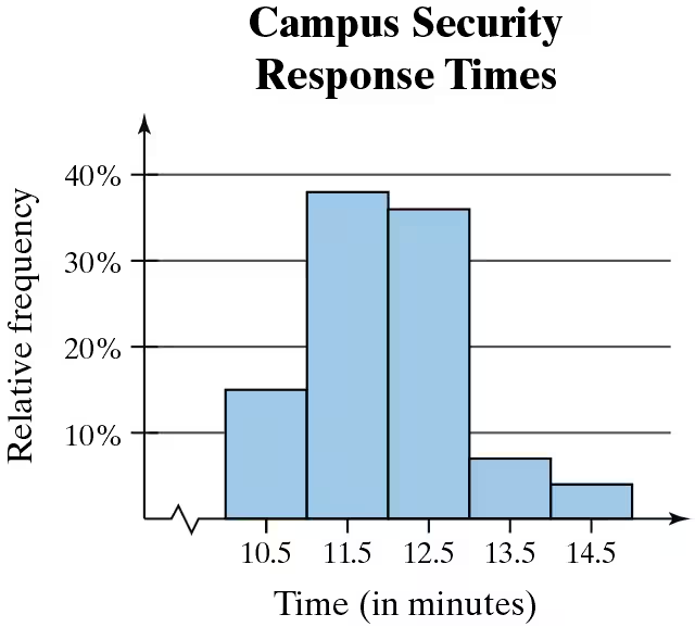
Use the relative frequency histogram to describe any patterns with the data.
Problem 2.1.46c
What Would You Do? The admissions department for a college is asked to recommend the minimum SAT scores that the college will accept for full-time students. The SAT scores of 50 applicants are listed. 1170 1000 910 870 1070 1290 920 1470 1080 1180 770 900 1120 1070 1370 1160 970 930 1240 1270 1250 1330 1010 1010 1410 1130 1210 1240 960 820 650 1010 1190 1500 1400 1270 1310 1050 950 1150 1450 1290 1310 1100 1330 1410 840 1040 1090 1080
If you want to accept the top 88% of the applicants, what should the minimum score be? Explain.
Problem 2.4.21c
Graphical Analysis In Exercises 21–24, you are asked to compare three data sets.
(c) Estimate the sample standard deviations. Then determine how close each of your estimates is by finding the sample standard deviations.
i.
ii.
iii.
Problem 2.1.27c
Use the ogive to approximate the
the number of black bears that weigh between 158.5 pounds and 244.5 pounds.
Problem 2.1.44c
Use the data set and the indicated number of classes to construct
(c) a frequency polygon,
Hospitals
Number of classes: 8
Data set: Number of hospitals in each of the 50 U.S. states and 5 inhabited territories (Source: American Hospital Directory) 10 90 51 1 77 341 56 34 8 214 111 3 14 40 18 142 102 55 75 108 72 53 19 105 55 83 1 69 19 108 10 27 14 78 37 31 186 146 90 37 177 52 11 67 25 100 361 35 91 2 7 61 78 33 14
Problem 2.1.45c
What Would You Do? You work at a bank and are asked to recommend the amount of cash to put in an ATM each day. You do not want to put in too much (which would cause security concerns) or too little (which may create customer irritation). The daily withdrawals (in hundreds of dollars) for 30 days are listed. 72 84 61 76 104 76 86 92 80 88 98 76 97 82 84 67 70 81 82 89 74 73 86 81 85 78 82 80 91 83
If you are willing to run out of cash on 10% of the days, how much cash should you put in the ATM each day? Explain.
Problem 2.5.11c
Using and Interpreting Concepts
Using and Interpreting Concepts Finding Quartiles, Interquartile Range, and Outliers In Exercises 11 and 12,
(c) identify any outliers.
56 63 51 60 57 60 60 54 63 59 80 63 60 62 65
Problem 2.5.27c
Studying Refer to the data set in Exercise 23 and the box-and-whisker plot you drew that represents the data set.
c. You randomly select one student from the sample. What is the likelihood that the student studied less than 2 hours per day? Write your answer as a percent.
Problem 2.4.55c
Pearson’s Index of Skewness The English statistician Karl Pearson (1857–1936) introduced a formula for the skewness of a distribution.
P = 3 (x̄ - median) / s
Most distributions have an index of skewness between -3 and 3. When P > 0, the data are skewed right. When P < 0, the data are skewed left. When P = 0, the data are symmetric. Calculate the coefficient of skewness for each distribution. Describe the shape of each.
c. x̄ = 9.2, s = 1.8, median = 9.2
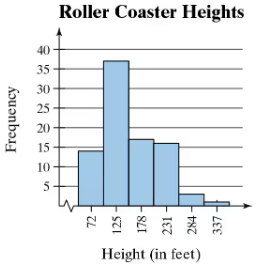
Problem 2.1.20d
Use the frequency histogram
describe any patterns with the data..
Problem 2.3.62d
Extending Concepts
Golf The distances (in yards) for nine holes of a golf course are listed.
336 393 408 522 147 504 177 375 360
d. Use your results from part (c) to explain how to quickly find the mean and the median of the original data set when the distances are converted to inches.
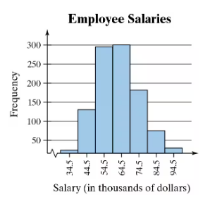
Problem 2.1.19d
Use the frequency histogram
d. describe any patterns with the data..
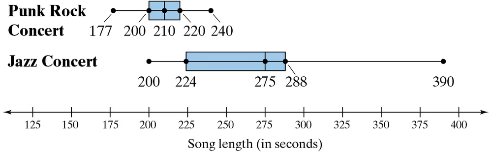
Problem 2.5.57d
Song Lengths Side-by-side box-and-whisker plots can be used to compare two or more different data sets. Each box-and-whisker plot is drawn on the same number line to compare the data sets more easily. The lengths (in seconds) of songs played at two different concerts are shown.
d. Can you determine which concert lasted longer? Explain.
Problem 2.4.55e
Pearson’s Index of Skewness The English statistician Karl Pearson (1857–1936) introduced a formula for the skewness of a distribution.
P = 3 (x̄ - median) / s
Most distributions have an index of skewness between -3 and 3. When P > 0, the data are skewed right. When P < 0, the data are skewed left. When P = 0, the data are symmetric. Calculate the coefficient of skewness for each distribution. Describe the shape of each.
e. x̄ = 155, s = 20.0, median = 175