Back
BackProblem 9.1.13b
Are Seat Belts Effective? A simple random sample of front-seat occupants involved in car crashes is obtained. Among 2823 occupants not wearing seat belts, 31 were killed. Among 7765 occupants wearing seat belts, 16 were killed (based on data from “Who Wants Airbags?” by Meyer and Finney, Chance, Vol. 18, No. 2). We want to use a 0.05 significance level to test the claim that seat belts are effective in reducing fatalities.
b. Test the claim by constructing an appropriate confidence interval.
Problem 9.2.9b
In Exercises 5–20, assume that the two samples are independent simple random samples selected from normally distributed populations, and do not assume that the population standard deviations are equal. (Note: Answers in Appendix D include technology answers based on Formula 9-1 along with “Table” answers based on Table A-3 with df equal to the smaller of n1-1 and n2-1)
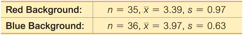
Color and Cognition Researchers from the University of British Columbia conducted a study to investigate the effects of color on cognitive tasks. Words were displayed on a computer screen with background colors of red and blue. Results from scores on a test of word recall are given below. Higher scores correspond to greater word recall.
b. Construct a confidence interval appropriate for the hypothesis test in part (a). What is it about the confidence interval that causes us to reach the same conclusion from part (a)?
Problem 9.2.18b
In Exercises 5–20, assume that the two samples are independent simple random samples selected from normally distributed populations, and do not assume that the population standard deviations are equal. (Note: Answers in Appendix D include technology answers based on Formula 9-1 along with “Table” answers based on Table A-3 with df equal to the smaller of n1-1 and n2-1)
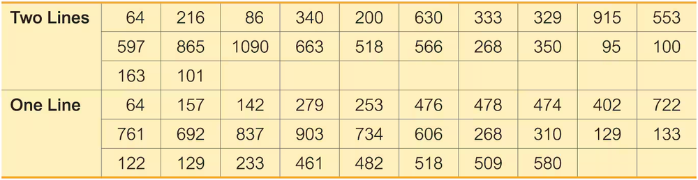
Queues Listed on the next page are waiting times (seconds) of observed cars at a Delaware inspection station. The data from two waiting lines are real observations, and the data from the single waiting line are modeled from those real observations. These data are from Data Set 30 “Queues” in Appendix B. The data were collected by the author.
b. Construct the confidence interval suitable for testing the claim in part (a).
Problem 9.2.6b
In Exercises 5–20, assume that the two samples are independent simple random samples selected from normally distributed populations, and do not assume that the population standard deviations are equal. (Note: Answers in Appendix D include technology answers based on Formula 9-1 along with “Table” answers based on Table A-3 with df equal to the smaller of n1-1 and n2-1)
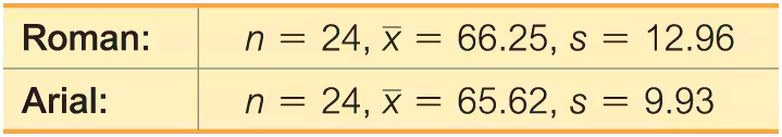
Readability of Font On a Computer Screen The statistics shown below were obtained from a standard test of readability of fonts on a computer screen (based on data from “Reading on the Computer Screen: Does Font Type Have Effects on Web Text Readability?” by Ali et al., International Education Studies, Vol. 6, No. 3). Reading speed and accuracy were combined into a readability performance score (x), where a higher score represents better font readability.
b. Construct the confidence interval suitable for testing the claim in part (a).
Problem 9.1.15b
Can Dogs Detect Malaria? A study was conducted to determine whether dogs could detect malaria from socks worn by malaria patients and socks worn by patients without malaria. Among 175 socks worn by malaria patients, the dogs made correct identifications 123 times. Among 145 socks worn by patients without malaria, the dogs made correct identifications 131 times (based on data presented at an annual meeting of the American Society of Tropical Medicine, by principal investigator Steve Lindsay). Use a 0.05 significance level to test the claim of no difference between the two rates of correct responses.
b. Test the claim by constructing an appropriate confidence interval.
Problem 9.2.13b
In Exercises 5–20, assume that the two samples are independent simple random samples selected from normally distributed populations, and do not assume that the population standard deviations are equal. (Note: Answers in Appendix D include technology answers based on Formula 9-1 along with “Table” answers based on Table A-3 with df equal to the smaller of n1-1 and n2-1)
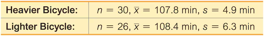
Bicycle Commuting A researcher used two different bicycles to commute to work. One bicycle was steel and weighed 30.0 lb; the other was carbon and weighed 20.9 lb. The commuting times (minutes) were recorded with the results shown below (based on data from “Bicycle Weights and Commuting Time,” by Jeremy Groves, British Medical Journal).
b. Construct the confidence interval suitable for testing the claim in part (a).
Problem 9.4.17b
Count Five Test for Comparing Variation in Two Populations Repeat Exercise 16 “Blanking Out on Tests,” but instead of using the F test, use the following procedure for the “count five” test of equal variations (which is not as complicated as it might appear).
b. Let c1 be the count of the number of absolute deviation values in the first sample that are greater than the largest absolute deviation value in the other sample. Also, let C2 be the count of the number of absolute deviation values in the second sample that are greater than the largest absolute deviation value in the other sample. (One of these counts will always be zero.)
Problem 9.3.7b
In Exercises 5–16, use the listed paired sample data, and assume that the samples are simple random samples and that the differences have a distribution that is approximately normal.
The Freshman 15 The “Freshman 15” refers to the belief that college students gain 15 lb (or 6.8 kg) during their freshman year. Listed below are weights (kg) of randomly selected male college freshmen (from Data Set 13 “Freshman 15” in Appendix B). The weights were measured in September and later in April.
b. Construct the confidence interval that could be used for the hypothesis test described in part (a). What feature of the confidence interval leads to the same conclusion reached in part (a)?
Problem 9.3.2b
Friday the 13th Refer to the sample data from Exercise 1.
b. In general, what does ud represent?
Problem 9.3.5b
In Exercises 5–16, use the listed paired sample data, and assume that the samples are simple random samples and that the differences have a distribution that is approximately normal.
Measured and Reported Weights Listed below are measured and reported weights (lb) of random female subjects (from Data Set 4 “Measured and Reported” in Appendix B).
b. Construct the confidence interval that could be used for the hypothesis test described in part (a). What feature of the confidence interval leads to the same conclusion reached in part (a)?
Problem 9.2.11b
In Exercises 5–20, assume that the two samples are independent simple random samples selected from normally distributed populations, and do not assume that the population standard deviations are equal. (Note: Answers in Appendix D include technology answers based on Formula 9-1 along with “Table” answers based on Table A-3 with df equal to the smaller of n1-1 and n2-1)
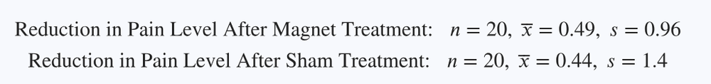
Magnet Treatment of Pain People spend around $5 billion annually for the purchase of magnets used to treat a wide variety of pains. Researchers conducted a study to determine whether magnets are effective in treating back pain. Pain was measured using the visual analog scale, and the results given below are among the results obtained in the study (based on data from “Bipolar Permanent Magnets for the Treatment of Chronic Lower Back Pain: A Pilot Study,” by Collacott, Zimmerman, White, and Rindone, Journal of the American Medical Association, Vol. 283, No. 10). Higher scores correspond to greater pain levels.
b. Construct the confidence interval appropriate for the hypothesis test in part (a).
Problem 9.2.10b
In Exercises 5–20, assume that the two samples are independent simple random samples selected from normally distributed populations, and do not assume that the population standard deviations are equal. (Note: Answers in Appendix D include technology answers based on Formula 9-1 along with “Table” answers based on Table A-3 with df equal to the smaller of n1-1 and n2-1)
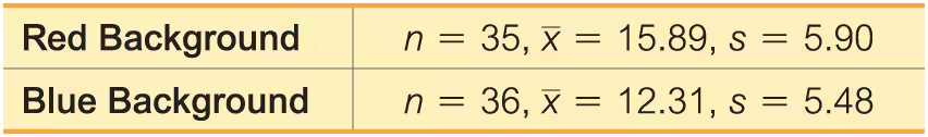
Color and Creativity Researchers from the University of British Columbia conducted trials to investigate the effects of color on creativity. Subjects with a red background were asked to think of creative uses for a brick; other subjects with a blue background were given the same task. Responses were scored by a panel of judges and results from scores of creativity are given below. Higher scores correspond to more creativity. The researchers make the claim that “blue enhances performance on a creative task.”
b. Construct the confidence interval appropriate for the hypothesis test in part (a). What is it about the confidence interval that causes us to reach the same conclusion from part (a)?
Problem 9.1.14b
Cigarette Pack Warnings A study was conducted to find the effects of cigarette pack warnings that consisted of text or pictures. Among 1078 smokers given cigarette packs with text warnings, 366 tried to quit smoking. Among 1071 smokers given cigarette packs with warning pictures, 428 tried to quit smoking. (Results are based on data from “Effect of Pictorial Cigarette Pack Warnings on Changes in Smoking Behavior,” by Brewer et al., Journal of the American Medical Association.) Use a 0.01 significance level to test the claim that the proportion of smokers who tried to quit in the text warning group is less than the proportion in the picture warning group.
b. Test the claim by constructing an appropriate confidence interval.
Problem 9.3.12b
In Exercises 5–16, use the listed paired sample data, and assume that the samples are simple random samples and that the differences have a distribution that is approximately normal.
Heights of Presidents A popular theory is that presidential candidates have an advantage if they are taller than their main opponents. Listed are heights (cm) of presidents along with the heights of their main opponents (from Data Set 22 “Presidents” in Appendix B).
b. Construct the confidence interval that could be used for the hypothesis test described in part (a). What feature of the confidence interval leads to the same conclusion reached in part (a)?
Problem 9.2.1b
Independent Samples Which of the following involve independent samples?
b. Data Set 6 “Births” includes birth weights of a sample of baby boys and a sample of baby girls.
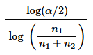
Problem 9.4.17c
Count Five Test for Comparing Variation in Two Populations Repeat Exercise 16 “Blanking Out on Tests,” but instead of using the F test, use the following procedure for the “count five” test of equal variations (which is not as complicated as it might appear).
c. If the sample sizes are equal (n1 = n2) use a critical value of 5. If n1 is not equals to n2 calculate the critical value shown below.
Problem 9.2.9c
In Exercises 5–20, assume that the two samples are independent simple random samples selected from normally distributed populations, and do not assume that the population standard deviations are equal. (Note: Answers in Appendix D include technology answers based on Formula 9-1 along with “Table” answers based on Table A-3 with df equal to the smaller of n1-1 and n2-1)
Color and Cognition Researchers from the University of British Columbia conducted a study to investigate the effects of color on cognitive tasks. Words were displayed on a computer screen with background colors of red and blue. Results from scores on a test of word recall are given below. Higher scores correspond to greater word recall.
c. Does the background color appear to have an effect on word recall scores? If so, which color appears to be associated with higher word memory recall scores?
Problem 9.1.12c
Clinical Trials of OxyContin OxyContin (oxycodone) is a drug used to treat pain, but it is well known for its addictiveness and danger. In a clinical trial, among subjects treated with OxyContin, 52 developed nausea and 175 did not develop nausea. Among other subjects given placebos, 5 developed nausea and 40 did not develop nausea (based on data from Purdue Pharma L.P.). Use a 0.05 significance level to test for a difference between the rates of nausea for those treated with OxyContin and those given a placebo.
c. Does nausea appear to be an adverse reaction resulting from OxyContin?
Problem 9.3.3c
Confidence Interval Assume that we want to use the sample data in Exercise 1 for constructing a confidence interval to be used for testing the given claim.
c. If the resulting confidence interval is -5.8 admissions <ud < -0.9 admissions, what do you conclude?
Problem 9.1.25c
Overlap of Confidence Intervals In the article “On Judging the Significance of Differences by Examining the Overlap Between Confidence Intervals,” by Schenker and Gentleman (American Statistician, Vol. 55, No. 3), the authors consider sample data in this statement: “Independent simple random samples, each of size 200, have been drawn, and 112 people in the first sample have the attribute, whereas 88 people in the second sample have the attribute.”
c. Use a 0.05 significance level to test the claim that the two population proportions are equal. What do you conclude?
Problem 9.4.1c
F Test Statistic
c. If testing the claim that sigma2,1 is not equals to sigma2,2 what do we know about the two samples if the test statistic F is very close to 1?
Problem 9.1.15c
Can Dogs Detect Malaria? A study was conducted to determine whether dogs could detect malaria from socks worn by malaria patients and socks worn by patients without malaria. Among 175 socks worn by malaria patients, the dogs made correct identifications 123 times. Among 145 socks worn by patients without malaria, the dogs made correct identifications 131 times (based on data presented at an annual meeting of the American Society of Tropical Medicine, by principal investigator Steve Lindsay). Use a 0.05 significance level to test the claim of no difference between the two rates of correct responses.
c. What do the results suggest about the use of dogs to detect malaria?
Problem 9.2.1c
Independent Samples Which of the following involve independent samples?
c. Data Set 1 “Body Data” includes a sample of pulse rates of 147 women and a sample of pulse rates of 153 men.
Problem 9.2.11c
In Exercises 5–20, assume that the two samples are independent simple random samples selected from normally distributed populations, and do not assume that the population standard deviations are equal. (Note: Answers in Appendix D include technology answers based on Formula 9-1 along with “Table” answers based on Table A-3 with df equal to the smaller of n1-1 and n2-1)
Magnet Treatment of Pain People spend around $5 billion annually for the purchase of magnets used to treat a wide variety of pains. Researchers conducted a study to determine whether magnets are effective in treating back pain. Pain was measured using the visual analog scale, and the results given below are among the results obtained in the study (based on data from “Bipolar Permanent Magnets for the Treatment of Chronic Lower Back Pain: A Pilot Study,” by Collacott, Zimmerman, White, and Rindone, Journal of the American Medical Association, Vol. 283, No. 10). Higher scores correspond to greater pain levels.
c. Does it appear that magnets are effective in treating back pain? Is it valid to argue that magnets might appear to be effective if the sample sizes are larger?
Problem 9.3.7c
In Exercises 5–16, use the listed paired sample data, and assume that the samples are simple random samples and that the differences have a distribution that is approximately normal.
The Freshman 15 The “Freshman 15” refers to the belief that college students gain 15 lb (or 6.8 kg) during their freshman year. Listed below are weights (kg) of randomly selected male college freshmen (from Data Set 13 “Freshman 15” in Appendix B). The weights were measured in September and later in April.
c. What do you conclude about the Freshman 15 belief?
Problem 9.1.13c
Are Seat Belts Effective? A simple random sample of front-seat occupants involved in car crashes is obtained. Among 2823 occupants not wearing seat belts, 31 were killed. Among 7765 occupants wearing seat belts, 16 were killed (based on data from “Who Wants Airbags?” by Meyer and Finney, Chance, Vol. 18, No. 2). We want to use a 0.05 significance level to test the claim that seat belts are effective in reducing fatalities.
c. What does the result suggest about the effectiveness of seat belts?
Problem 9.4.1d
F Test Statistic
d. Is the F distribution symmetric, skewed left, or skewed right?
Problem 9.4.17d
Count Five Test for Comparing Variation in Two Populations Repeat Exercise 16 “Blanking Out on Tests,” but instead of using the F test, use the following procedure for the “count five” test of equal variations (which is not as complicated as it might appear).
d. If c1 equal to or greater than critical value then conclude that sigma2,1 > sigma2,2 If c1 equal to or greater than critical value then conclude that sigma2,2 > sigma2,1. Otherwise, fail to reject the null hypothesis of sigma2,1 = sigma2,2
Problem 9.q.3a
P-VALUE The test statistic of z = 2.14 is obtained when using the data from Exercise 1 and testing the claim that patients treated with dexamethasone and patients given a placebo have the same rate of complete resolution.
a. Find the P-value for the test.
Problem 10a
Denomination Effect A trial was conducted with 75 women in China given a 100-yuan bill, while another 75 women in China were given 100 yuan in the form of smaller bills (a 50-yuan bill plus two 20-yuan bills plus two 5-yuan bills). Among those given the single bill, 60 spent some or all of the money. Among those given the smaller bills, 68 spent some or all of the money (based on data from “The Denomination Effect,” by Raghubir and Srivastava, Journal of Consumer Research, Vol. 36). We want to use a 0.05 significance level to test the claim that when given a single large bill, a smaller proportion of women in China spend some or all of the money when compared to the proportion of women in China given the same amount in smaller bills.
a. Test the claim using a hypothesis test.