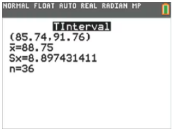
In Exercises 1–4, refer to the accompanying screen display that results from a simple random sample of times (minutes) between eruptions of the Old Faithful geyser. The confidence level of 95% was used.

Refer to the accompanying screen display.

a. Express the confidence interval in the format that uses the “less than” symbol. Round the confidence interval limits given that the original times are all rounded to one decimal place.

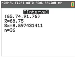
In Exercises 1–4, refer to the accompanying screen display that results from a simple random sample of times (minutes) between eruptions of the Old Faithful geyser. The confidence level of 95% was used.

Degrees of Freedom

a. What is the number of degrees of freedom that should be used for finding the critical value ta/2?

In Exercises 1–4, refer to the accompanying screen display that results from a simple random sample of times (minutes) between eruptions of the Old Faithful geyser. The confidence level of 95% was used.

Degrees of Freedom

b. Find the critical value ta/2 corresponding to a 95% confidence level.

In Exercises 1–4, refer to the accompanying screen display that results from a simple random sample of times (minutes) between eruptions of the Old Faithful geyser. The confidence level of 95% was used.

Interpreting a Confidence Interval The results in the screen display are based on a 95% confidence level. Write a statement that correctly interprets the confidence interval.

In Exercises 5–8, (a) identify the critical value ta/2 used for finding the margin of error, (b) find the margin of error, (c) find the confidence interval estimate of u, and (d) write a brief statement that interprets the confidence interval.

Birth Weights Here are summary statistics for randomly selected weights of newborn girls: n=36, x=3150.0g, s=695.5g (based on Data Set 6 “Births” in Appendix B). Use a confidence level of 95%.

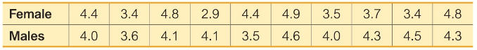
Professor Evaluation Scores Listed below are student evaluation scores of professors from Data Set 28 “Course Evaluations” in Appendix B. Construct a 95% confidence interval estimate of for each of the two data sets. Does there appear to be a difference in variation?

Heights of Presidents Refer to Data Set 22 “Presidents” in Appendix B. Treat the data as a sample and find the proportion of presidents who were taller than their opponents. Use that result to construct a 95% confidence interval estimate of the population percentage. Based on the result, does it appear that greater height is an advantage for presidential candidates? Why or why not?

Constructing and Interpreting Confidence Intervals. In Exercises 13–16, use the given sample data and confidence level. In each case, (a) find the best point estimate of the population proportion p; (b) identify the value of the margin of error E; (c) construct the confidence interval; (d) write a statement that correctly interprets the confidence interval.

Medical Malpractice In a study of 1228 randomly selected medical malpractice lawsuits, it was found that 856 of them were dropped or dismissed (based on data from the Physicians Insurers Association of America). Construct a 95% confidence interval for the proportion of medical malpractice lawsuits that are dropped or dismissed.

Body Temperature Data Set 5 “Body Temperatures” in Appendix B includes a sample of 106 body temperatures having a mean of and a standard deviation of 0.62F (for day 2 at 12 AM). Construct a 95% confidence interval estimate of the standard deviation of the body temperatures for the entire population.

Finding Critical Values

In Exercises 5–8, find the critical value z=a/2 that corresponds to the given confidence level.

99.5%

Mercury in Sushi An FDA guideline is that the mercury in fish should be below 1 part per million (ppm). Listed below are the amounts of mercury (ppm) found in tuna sushi sampled at different stores in New York City. The study was sponsored by the New York Times, and the stores (in order) are D’Agostino, Eli’s Manhattan, Fairway, Food Emporium, Gourmet Garage, Grace’s Marketplace, and Whole Foods. Construct a 98% confidence interval estimate of the mean amount of mercury in the population. Does it appear that there is too much mercury in tuna sushi?

0.56 0.75 0.10 0.95 1.25 0.54 0.88

Los Angeles Commute Time Listed below are 15 Los Angeles commute times (based on a sample from Data Set 31 “Commute Times” in Appendix B). Construct a 99% confidence interval estimate of the population mean. Is the confidence interval a good estimate of the population mean?

In Exercises 5–8, (a) identify the critical value ta/2 used for finding the margin of error, (b) find the margin of error, (c) find the confidence interval estimate of u, and (d) write a brief statement that interprets the confidence interval.

Pepsi Weights Here are summary statistics for the weights of Pepsi in randomly selected cans: n=36, x=0.82410 lb, s=0.00570 lb (based on Data Set 37 “Cola Weights and Volumes” in Appendix B). Use a confidence level of 99%.

Finding Critical Values.

In Exercises 5–8, find the critical value z=a/2 that corresponds to the given confidence level.

90%

Constructing and Interpreting Confidence Intervals. In Exercises 13–16, use the given sample data and confidence level. In each case, (a) find the best point estimate of the population proportion p; (b) identify the value of the margin of error E; (c) construct the confidence interval; (d) write a statement that correctly interprets the confidence interval.

Tennis Challenges In a recent U.S. Open tennis tournament, men playing singles matches used challenges on 240 calls made by the line judges. Among those challenges, 88 were found to be successful with the call overturned. Construct a 95% confidence interval for the proportion of successful challenges.

Large Data Sets from Appendix B. In Exercises 21 and 22, use the data set in Appendix B. Assume that each sample is a simple random sample obtained from a population with a normal distribution.

Comparing Waiting Lines Refer to Data Set 30 “Queues” in Appendix B. Construct separate 95% confidence interval estimates of using the two-line wait times and the single-line wait times. Do the results support the expectation that the single line has less variation? Do the wait times from both line configurations satisfy the requirements for confidence interval estimates of sigma

Second-Hand Smoke Refer to Data Set 15 “Passive and Active Smoke” and construct a 95% confidence interval estimates of the mean cotinine level in each of three samples: (1) people who smoke; (2) people who don’t smoke but are exposed to tobacco smoke at home or work; (3) people who don’t smoke and are not exposed to smoke. Measuring cotinine in people’s blood is the most reliable way to determine exposure to nicotine. What do the confidence intervals suggest about the effects of smoking and second-hand smoke?

Confidence Levels

Given specific sample data, such as the data given in Exercise 1, which confidence interval is wider: the 95% confidence interval or the 80% confidence interval? Why is it wider?

Mean IQ of Data Scientists See the preceding exercise, in which we can assume that sigma=15 for the IQ scores. Data scientists are a group with IQ scores that vary less than the IQ scores of the general population. Find the sample size needed to estimate the mean IQ of data scientists, given that we want 98% confidence that the sample mean is within 2 IQ points of the population mean. Does the sample size appear to be practical?

Seating Choice In a 3M Privacy Filters poll, respondents were asked to identify their favorite seat when they fly, and the results include these responses: window, window, other, other. Letting “window” and letting “other”, those four responses can be represented as {1, 1, 0, 0}. Here are ten bootstrap samples for those responses: [Image]

Using only the ten given bootstrap samples, construct an 80% confidence interval estimate of the proportion of respondents who indicated their favorite seat is “window.”

Formats of Confidence Intervals. In Exercises 9–12, express the confidence interval using the indicated format. (The confidence intervals are based on the proportions of red, orange, yellow, and blue M&Ms in Data Set 38 “Candies” in Appendix B.)

Green M&Ms Express 0.116 < p < 0.192 in the form of p +-E.

Sample Size for Proportion Find the sample size required to estimate the percentage of statistics students who take their statistics course online. Assume that we want 95% confidence that the proportion from the sample is within two percentage points of the true population percentage.

Atkins Weight Loss Program In a test of weight loss programs, 40 adults used the Atkins weight loss program. After 12 months, their mean weight loss was found to be 2.1 lb, with a standard deviation of 4.8 lb. Construct a 90% confidence interval estimate of the standard deviation of the weight loss for all such subjects. Does the confidence interval give us information about the effectiveness of the diet?

Genes Samples of DNA are collected, and the four DNA bases of A, G, C, and T are coded as 1, 2, 3, and 4, respectively. The results are listed below. Construct a 95% confidence interval estimate of the mean. What is the practical use of the confidence interval?

2 2 1 4 3 3 3 3 4 1

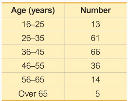
Ages of Prisoners The accompanying frequency distribution summarizes sample data consisting of ages of randomly selected inmates in federal prisons (based on data from the Federal Bureau of Prisons). Use the data to construct a 95% confidence interval estimate of the mean age of all inmates in federal prisons.

Estimating the Median Use the sample data listed in Exercise 1 “Bootstrap Requirements” to generate 1000 bootstrap samples, and find the median in each of those samples. After obtaining the 1000 sample medians, find the 95% confidence interval estimate of the population median by evaluating p2.5 and p97.5 from the sorted 1000 medians. Given that the sample times in Exercise 1 are from the 50 times in Data Set 20 “Alcohol and Tobacco in Movies” and those 50 times have a median of 5.5, how well did the bootstrap method work to create a “good” confidence interval?

Female Motorcycle Owners Here is a 95% confidence interval estimate of the percentage of motorcycle owners who are female: 17.5%<p<20.6% (based on data from the Motorcycle Industry Council). What is the best point estimate of the percentage of motorcycle owners who are women?

Mean Assume that we want to use the sample data given in Exercise 1 with the bootstrap method to estimate the population mean. The mean of the values in Exercise 1 is 54.3 seconds, and the mean of all of the tobacco times in Data Set 20 “Alcohol and Tobacco in Movies” from Appendix B is 57.4 seconds. If we use 1000 bootstrap samples and find the corresponding 1000 means, do we expect that those 1000 means will target 54.3 seconds or 57.4 seconds? What does that result suggest about the bootstrap method in this case?

Ages of Moviegoers Find the sample size needed to estimate the mean age of movie patrons, given that we want 98% confidence that the sample mean is within 1.5 years of the population mean. Assume that sigma=19.6 years, based on a previous report from the Motion Picture Association of America. Could the sample be obtained from one movie at one theater?

Critical Thinking. In Exercises 17–28, use the data and confidence level to construct a confidence interval estimate of p, then address the given question.

Births A random sample of 860 births in New York State included 426 boys. Construct a 95% confidence interval estimate of the proportion of boys in all births. It is believed that among all births, the proportion of boys is 0.512. Do these sample results provide strong evidence against that belief?