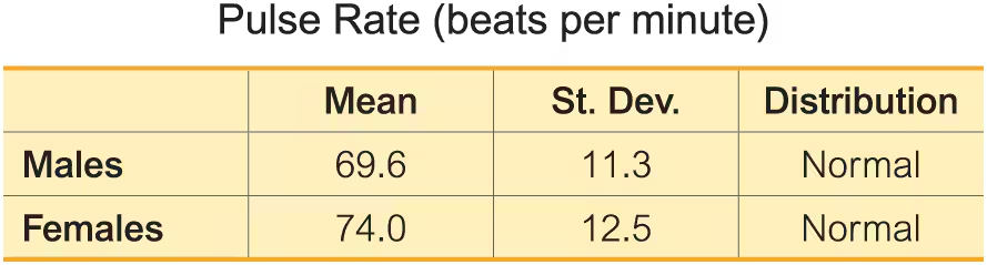
Pulse Rates. In Exercises 13–24, use the data in the table below for pulse rates of adult males and females (based on Data Set 1 “Body Data” in Appendix B). Hint: Draw a graph in each case.

For males, find P90 which is the pulse rate separating the bottom 90% from the top 10%.

In Exercises 1 and 2, use the following wait times (minutes) at 10:00 AM for the Tower of Terror ride at Disney World (from Data Set 33 “Disney World Wait Times” in Appendix B).

35 35 20 50 95 75 45 50 30 35 30 30

h. Are the wait times discrete data or continuous data?

Foot Lengths of Women Assume that foot lengths of adult females are normally distributed with a mean of 246.3 mm and a standard deviation of 12.4 mm (based on Data Set 3 “ANSUR II 2012” in Appendix B).

c. Find P95.

Foot Lengths of Women Assume that foot lengths of adult females are normally distributed with a mean of 246.3 mm and a standard deviation of 12.4 mm (based on Data Set 3 “ANSUR II 2012” in Appendix B).

a. Find the probability that a randomly selected adult female has a foot length less than 221.5 mm.

Normal Distribution Using a larger data set than the one given for the preceding exercises, assume that cell phone radiation amounts are normally distributed with a mean of 1.17 W/kg and a standard deviation of 0.29 W/kg.

a. Find the probability that a randomly selected cell phone has a radiation amount that exceeds the U.S. standard of 1.6 W/kg or less.

Blue Eyes Assume that 35% of us have blue eyes (based on a study by Dr. P. Soria at Indiana University).

b. Find the value of P(B_bar).

In Exercises 1 and 2, use the following wait times (minutes) at 10:00 AM for the Tower of Terror ride at Disney World (from Data Set 33 “Disney World Wait Times” in Appendix B).

35 35 20 50 95 75 45 50 30 35 30 30

e. Convert the longest wait time to a z score.

f. Based on the result from part (e), is the longest wait time significantly high?

Blue Eyes Assume that 35% of us have blue eyes (based on a study by Dr. P. Soria at Indiana University).

c. Find the probability of randomly selecting three different people and finding that all of them have blue eyes.

In Exercises 1 and 2, use the following wait times (minutes) at 10:00 AM for the Tower of Terror ride at Disney World (from Data Set 33 “Disney World Wait Times” in Appendix B).

35 35 20 50 95 75 45 50 30 35 30 30

b. Construct a boxplot.

In Exercises 1 and 2, use the following wait times (minutes) at 10:00 AM for the Tower of Terror ride at Disney World (from Data Set 33 “Disney World Wait Times” in Appendix B).

35 35 20 50 95 75 45 50 30 35 30 30 

b. Find the median.

Foot Lengths of Women Assume that foot lengths of adult females are normally distributed with a mean of 246.3 mm and a standard deviation of 12.4 mm (based on Data Set 3 “ANSUR II 2012” in Appendix B).

d. Find the probability that 16 adult females have foot lengths with a mean greater than 250 mm.

In Exercises 1 and 2, use the following wait times (minutes) at 10:00 AM for the Tower of Terror ride at Disney World (from Data Set 33 “Disney World Wait Times” in Appendix B).

35 35 20 50 95 75 45 50 30 35 30 30

a. Find the mean xbar.

In Exercises 1 and 2, use the following wait times (minutes) at 10:00 AM for the Tower of Terror ride at Disney World (from Data Set 33 “Disney World Wait Times” in Appendix B).

35 35 20 50 95 75 45 50 30 35 30 30

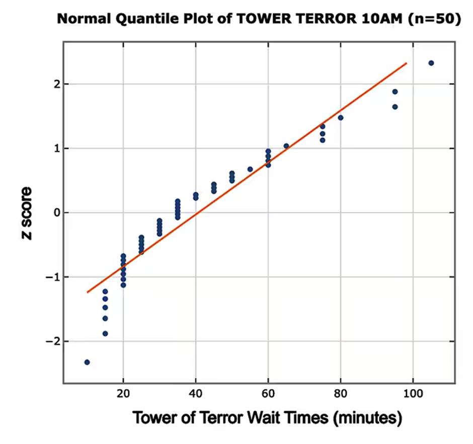
d. The accompanying normal quantile plot is obtained by using all 50 wait times at 10:00 AM for the Tower of Terror ride at Disney World. Based on this normal quantile plot, do the sample data appear to be from a normally distributed population?

Bone Density Test A bone mineral density test is used to identify a bone disease. The result of a bone density test is commonly measured as a z score, and the population of z scores is normally distributed with a mean of 0 and a standard deviation of 1.

e. If the mean bone density test score is found for 9 randomly selected subjects, find the probability that the mean is greater than 0.23.

Arm Circumferences Arm circumferences of adult men are normally distributed with a mean of 33.64 cm and a standard deviation of 4.14 cm (based on Data Set 1 “Body Data” in Appendix B). A sample of 25 men is randomly selected and the mean of the arm circumferences is obtained.

b. What is the mean of all such sample means?

In Exercises 8 and 9, assume that women have standing eye heights that are normally distributed with a mean of 59.7 in. and a standard deviation of 2.5 in. (based on anthropometric survey data from Gordon, Churchill, et al.).

a. If an eye recognition security system is positioned at a height that is uncomfortable for women with standing eye heights less than 54 in., what percentage of women will find that height uncomfortable?

Mensa Membership in Mensa requires a score in the top 2% on a standard intelligence test. The Wechsler IQ test is designed for a mean of 100 and a standard deviation of 15, and scores are normally distributed.

a. Find the minimum Wechsler IQ test score that satisfies the Mensa requirement.

Mensa Membership in Mensa requires a score in the top 2% on a standard intelligence test. The Wechsler IQ test is designed for a mean of 100 and a standard deviation of 15, and scores are normally distributed.

b. If 4 randomly selected adults take the Wechsler IQ test, find the probability that their mean score is at least 131.

Birth Weights Based on Data Set 6 “Births” in Appendix B, birth weights of girls are normally distributed with a mean of 3037.1 g and a standard deviation of 706.3 g.

c. What is the value of the mode?

Birth Weights Based on Data Set 6 “Births” in Appendix B, birth weights of girls are normally distributed with a mean of 3037.1 g and a standard deviation of 706.3 g.

b. What is the value of the median?

In Exercises 8 and 9, assume that women have standing eye heights that are normally distributed with a mean of 59.7 in. and a standard deviation of 2.5 in. (based on anthropometric survey data from Gordon, Churchill, et al.).

Significance Instead of using 0.05 for identifying significant values, use the criteria that a value x is significantly high if P(x or greater) ≤ 0.01 and a value is significantly low if P(x or less) ≤ 0.01. Find the standing eye heights of women that separate significant values from those that are not significant. Using these criteria, is a woman’s standing eye height of 67 in. significantly high?

Mensa Membership in Mensa requires a score in the top 2% on a standard intelligence test. The Wechsler IQ test is designed for a mean of 100 and a standard deviation of 15, and scores are normally distributed.

c. If 4 subjects take the Wechsler IQ test and they have a mean of 131 but the individual scores are lost, can we conclude that all 4 of them have scores of at least 131?

Fatal Car Crashes There are about 15,000 car crashes each day in the United States, and the proportion of car crashes that are fatal is 0.00559 (based on data from the National Highway Traffic Safety Administration). Assume that each day, 1000 car crashes are randomly selected and the proportion of fatal car crashes is recorded.

a. What do you know about the mean of the sample proportions?

Sleepwalking Assume that 29.2% of people have sleepwalked (based on “Prevalence and Comorbidity of Nocturnal Wandering in the U.S. Adult General Population, by Ohayon et al., Neurology, Vol. 78, No. 20). Assume that in a random sample of 1480 adults, 455 have sleepwalked.

a. Assuming that the rate of 29.2% is correct, find the probability that 455 or more of the 1480 adults have sleepwalked.

Using the Central Limit Theorem. In Exercises 5–8, assume that the amounts of weight that male college students gain during their freshman year are normally distributed with a mean of 1.2 kg and a standard deviation of 4.9 kg (based on Data Set 13 “Freshman 15” in Appendix B).

a. If 1 male college student is randomly selected, find the probability that he gains at least 2.0 kg during his freshman year..)

Ergonomics. Exercises 9–16 involve applications to ergonomics, as described in the Chapter Problem.

Doorway Height The Boeing 757-200 ER airliner carries 200 passengers and has doors with a height of 72 in. Heights of men are normally distributed with a mean of 68.6 in. and a standard deviation of 2.8 in. (based on Data Set 1 “Body Data” in Appendix B).

a. If a male passenger is randomly selected, find the probability that he can fit through the doorway without bending.

College Presidents There are about 4200 college presidents in the United States, and they have annual incomes with a distribution that is skewed instead of being normal. Many different samples of 40 college presidents are randomly selected, and the mean annual income is computed for each sample.

a. What is the approximate shape of the distribution of the sample means (uniform, normal, skewed, other)?

Ergonomics. Exercises 9–16 involve applications to ergonomics, as described in the Chapter Problem.

Safe Loading of Elevators The elevator in the car rental building at San Francisco International Airport has a placard stating that the maximum capacity is “4000 lb—27 passengers.” Because 4000/27=148, this converts to a mean passenger weight of 148 lb when the elevator is full. We will assume a worst-case scenario in which the elevator is filled with 27 adult males. Based on Data Set 1 “Body Data” in Appendix B, assume that adult males have weights that are normally distributed with a mean of 189 lb and a standard deviation of 39 lb.

a. Find the probability that 1 randomly selected adult male has a weight greater than 148 lb.

Body Temperatures Listed below are body temperatures (°F) of adult males (based on Data Set 5 “Body Temperatures” in Appendix B).

97.6 98.2 99.6 98.7 99.4 98.2 98.0 98.6 98.6

a. Find the mean. Does the result seem reasonable?

Using the Central Limit Theorem. In Exercises 5–8, assume that the amounts of weight that male college students gain during their freshman year are normally distributed with a mean of 1.2 kg and a standard deviation of 4.9 kg (based on Data Set 13 “Freshman 15” in Appendix B).

a. If 1 male college student is randomly selected, find the probability that he gains between 0.5 kg and 2.5 kg during freshman year.