Determining Normality. In Exercises 9–12, refer to the indicated sample data and determine whether they appear to be from a population with a normal distribution. Assume that this requirement is loose in the sense that the population distribution need not be exactly normal, but it must be a distribution that is roughly bell-shaped.

Taxi Trips The distances (miles) traveled by New York City taxis transporting customers, as listed in Data Set 32 “Taxis” in Appendix B

Outliers For the purposes of constructing modified boxplots as described in Section 3-3, outliers are defined as data values that are above Q3 by an amount greater than 1.5 x IQR or below Q1 by an amount greater than 1.5 x IQR, where IQR is the interquartile range. Using this definition of outliers, find the probability that when a value is randomly selected from a normal distribution, it is an outlier.

Determining Normality. In Exercises 9–12, refer to the indicated sample data and determine whether they appear to be from a population with a normal distribution. Assume that this requirement is loose in the sense that the population distribution need not be exactly normal, but it must be a distribution that is roughly bell-shaped.

Dunkin’ Donuts The drive-through service times (seconds) of Dunkin’ Donuts lunch customers, as listed in Data Set 36 “Fast Food” in Appendix B

Good Sample? An economist is investigating the incomes of college students. Because she lives in Maine, she obtains sample data from that state. Is the resulting mean income of college students a good estimator of the mean income of college students in the United States? Why or why not?

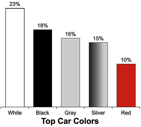
Car Colors

In Exercises 9–12, assume that 100 cars are randomly selected. Refer to the accompanying graph, which shows the top car colors and the percentages of cars with those colors (based on PPG Industries).

Black Cars Find the probability that at least 25 cars are black. Is 25 a significantly high number of black cars?

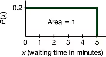
Continuous Uniform Distribution. In Exercises 5–8, refer to the continuous uniform distribution depicted in Figure 6-2 and described in Example 1. Assume that a passenger is randomly selected, and find the probability that the waiting time is within the given range.

Greater than 3.00 minutes

Basis for the Range Rule of Thumb and the Empirical Rule. In Exercises 45–48, find the indicated area under the curve of the standard normal distribution; then convert it to a percentage and fill in the blank. The results form the basis for the range rule of thumb and the empirical rule introduced in Section 3-2.

About __ % of the area is between z = -3.5 and z = 3.5 (or within 3.5 standard deviation of the mean).

Births: Sampling Distribution of Sample Proportion When two births are randomly selected, the sample space for genders is bb, bg, gb, and gg (where and Assume that those four outcomes are equally likely. Construct a table that describes the sampling distribution of the sample proportion of girls from two births. Does the mean of the sample proportions equal the proportion of girls in two births? Does the result suggest that a sample proportion is an unbiased estimator of a population proportion?

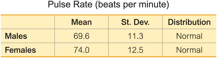
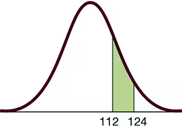
Pulse Rates. In Exercises 13–24, use the data in the table below for pulse rates of adult males and females (based on Data Set 1 “Body Data” in Appendix B). Hint: Draw a graph in each case.

Find the probability that a male has a pulse rate between 70 beats per minute and 90 beats per minute.

Standard Normal Distribution. In Exercises 17–36, assume that a randomly selected subject is given a bone density test. Those test scores are normally distributed with a mean of 0 and a standard deviation of 1. In each case, draw a graph, then find the probability of the given bone density test scores. If using technology instead of Table A-2, round answers to four decimal places.

Less than -2.00

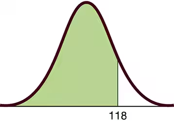
Pulse Rates. In Exercises 13–24, use the data in the table below for pulse rates of adult males and females (based on Data Set 1 “Body Data” in Appendix B). Hint: Draw a graph in each case.

For males, find P90 which is the pulse rate separating the bottom 90% from the top 10%.

Critical Values. In Exercises 41–44, find the indicated critical value. Round results to two decimal places.

z0.90

IQ Scores. In Exercises 5–8, find the area of the shaded region. The graphs depict IQ scores of adults, and those scores are normally distributed with a mean of 100 and a standard deviation of 15 (as on the Wechsler IQ test).

Small Sample Weights of M&M plain candies are normally distributed. Twelve M&M plain candies are randomly selected and weighed, and then the mean of this sample is calculated. Is it correct to conclude that the resulting sample mean cannot be considered to be a value from a normally distributed population because the sample size of 12 is too small? Explain.

IQ Scores. In Exercises 5–8, find the area of the shaded region. The graphs depict IQ scores of adults, and those scores are normally distributed with a mean of 100 and a standard deviation of 15 (as on the Wechsler IQ test).

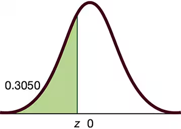
Standard Normal Distribution. In Exercises 13–16, find the indicated z score. The graph depicts the standard normal distribution of bone density scores with mean 0 and standard deviation 1.

Finding Bone Density Scores. In Exercises 37–40 assume that a randomly selected subject is given a bone density test. Bone density test scores are normally distributed with a mean of 0 and a standard deviation of 1. In each case, draw a graph, then find the bone density test score corresponding to the given information. Round results to two decimal places.

Find the bone density scores that are the quartiles Q1, Q2, and Q3.

Interpreting Normal Quantile Plots. In Exercises 5–8, examine the normal quantile plot and determine whether the sample data appear to be from a population with a normal distribution.

Ages of Presidents The normal quantile plot represents the ages of presidents of the United States at the times of their inaugurations. The data are from Data Set 22 “Presidents” in Appendix B.

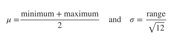
Distributions In a continuous uniform distribution,

a. Find the mean and standard deviation for the distribution of the waiting times represented in Figure 6-2, which accompanies Exercises 5–8.

Satisfying Requirements Data Set 1 “Body Data” in Appendix B includes a sample of 147 pulse rates of randomly selected women. Does that sample satisfy the following requirement: (1) The sample appears to be from a normally distributed population; or (2) the sample has a size of n>30?

Continuous Uniform Distribution. In Exercises 5–8, refer to the continuous uniform distribution depicted in Figure 6-2 and described in Example 1. Assume that a passenger is randomly selected, and find the probability that the waiting time is within the given range.

Between 2 minutes and 3 minutes

Basis for the Range Rule of Thumb and the Empirical Rule. In Exercises 45–48, find the indicated area under the curve of the standard normal distribution; then convert it to a percentage and fill in the blank. The results form the basis for the range rule of thumb and the empirical rule introduced in Section 3-2.

About __ % of the area is between z = -1 and z = 1 (or within 1 standard deviation of the mean).

Standard Normal Distribution. In Exercises 9–12, find the area of the shaded region. The graph depicts the standard normal distribution of bone density scores with mean 0 and standard deviation 1.

Tennis Replay In a recent year, there were 879 challenges made to referee calls in professional tennis singles play. Among those challenges, 231 challenges were upheld with the call overturned. Assume that in general, 25% of the challenges are successfully upheld with the call overturned.

a. If the 25% rate is correct, find the probability that among the 879 challenges, the number of overturned calls is exactly 231.

Overbooking a Boeing 767-300 A Boeing 767-300 aircraft has 213 seats. When someone buys a ticket for a flight, there is a 0.0995 probability that the person will not show up for the flight (based on data from an IBM research paper by Lawrence, Hong, and Cherrier). How many reservations could be accepted for a Boeing 767-300 for there to be at least a 0.95 probability that all reservation holders who show will be accommodated?

Constructing Normal Quantile Plots. In Exercises 17–20, use the given data values to identify the corresponding z scores that are used for a normal quantile plot, then identify the coordinates of each point in the normal quantile plot. Construct the normal quantile plot, then determine whether the data appear to be from a population with a normal distribution.

Earthquake Depths A sample of depths (km) of earthquakes is obtained from Data Set 24 “Earthquakes” in Appendix B: 17.3, 7.0, 7.0, 7.0, 8.1, 6.8.

Standard Normal Distribution. In Exercises 17–36, assume that a randomly selected subject is given a bone density test. Those test scores are normally distributed with a mean of 0 and a standard deviation of 1. In each case, draw a graph, then find the probability of the given bone density test scores. If using technology instead of Table A-2, round answers to four decimal places.

Between 1.50 and 2.00

Continuous Uniform Distribution. In Exercises 5–8, refer to the continuous uniform distribution depicted in Figure 6-2 and described in Example 1. Assume that a passenger is randomly selected, and find the probability that the waiting time is within the given range.

Less than 4.00 minutes

Hypothesis Testing. In Exercises 17–19, apply the central limit theorem to test the given claim. (Hint: See Example 3.)

Adult Sleep Times (hours) of sleep for randomly selected adult subjects included in the National Health and Nutrition Examination Study are listed below. Here are the statistics for this sample: n = 12, x_bar = 6.8 hours, s = 20 hours. The times appear to be from a normally distributed population. A common recommendation is that adults should sleep between 7 hours and 9 hours each night. Assuming that the mean sleep time is 7 hours, find the probability of getting a sample of 12 adults with a mean of 6.8 hours or less. What does the result suggest about a claim that “the mean sleep time is less than 7 hours”?

4 8 4 4 8 6 9 7 7 10 7 8

Notation Common tests such as the SAT, ACT, LSAT, and MCAT tests use multiple choice test questions, each with possible answers of a, b, c, d, e, and each question has only one correct answer. For people who make random guesses for answers to a block of 100 questions, identify the values of p, q, μ, and σ. What do μ and σ measure?