Back
BackProblem 2.T.8b
The mean gestational length of a sample of 208 horses is 343.7 days, with a standard deviation of 10.4 days. The data set has a bell-shaped distribution.
b. Determine whether a gestational length of 318.4 days is unusual.
Problem 2.T.3
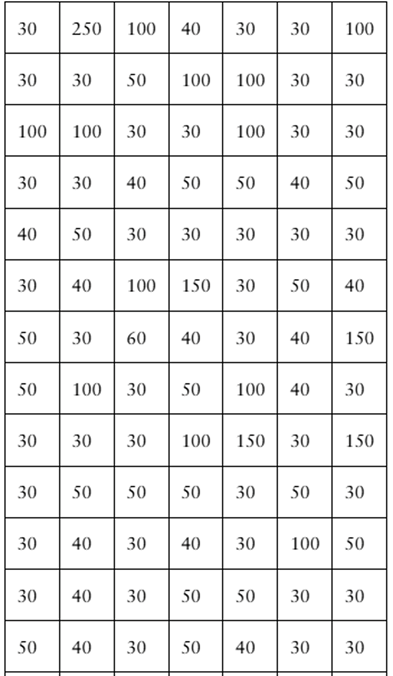
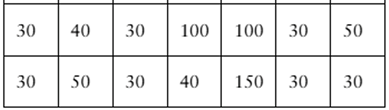
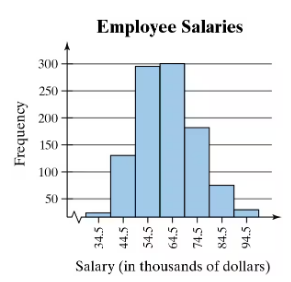
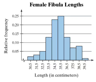
Use frequency distribution formulas to estimate the sample mean and the sample standard deviation of the data set in Exercise 2.
Problem 2.T.1
According to data from the city of Toronto, Ontario, Canada, there were nearly 112,000 parking infractions in the city for December 2020, with fines totaling over 5,500,000 Canadian dollars. The fines (in Canadian dollars) for a random sample of 105 parking infractions in Toronto, Ontario, Canada, for December 2020 are listed below. (Source: City of Toronto)
In Exercises 1–5, use technology. If possible, print your results.
Find the sample mean of the data.
Problem 2.T.2b
The data set represents the number of movies that a sample of 20 people watched in a year.
121 148 94 142 170 88 221 106 18 67
149 28 60 101 134 168 92 154 53 66
b. Display the data using a frequency histogram and a frequency polygon on the same axes.
Problem 2.4.31a
Using the Empirical Rule In Exercises 29–34, use the Empirical Rule.
Use the sample statistics from Exercise 29 and assume the number of vehicles in the sample is 75.
a. Estimate the number of vehicles whose speeds are between 63 miles per hour and 71 miles per hour.
Problem 2.3.57a
Protein Powder During a quality assurance check, the actual contents (in grams) of six containers of protein powder were recorded as 1525, 1526, 1502, 1516, 1529, and 1511.
a. Find the mean and the median of the contents.
Problem 2.1.26a
use the ogive to approximate
the number in the sample.
Problem 2.3.62a
Extending Concepts
Golf The distances (in yards) for nine holes of a golf course are listed.
336 393 408 522 147 504 177 375 360
a. Find the mean and the median of the data.
Problem 2.3.66a
Extending Concepts
Trimmed Mean To find the 10% trimmed mean of a data set, order the data, delete the lowest 10% of the entries and the highest 10% of the entries, and find the mean of the remaining entries.
a. Find the 10% trimmed mean for the data in Exercise 65.
Problem 2.3.58a
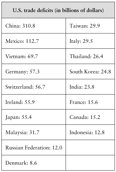
U.S. Trade Deficits The table at the left shows the U.S. trade deficits (in billions of dollars) with 18 countries in 2020. (Source: U.S. Department of Commerce)
a. Find the mean and the median of the trade deficits.
Problem 2.5.18a
Drawing a Box-and-Whisker Plot In Exercises 15–18,
(a) find the five-number summary
2 7 1 3 1 2 8 9 9 2 5 4 7 3 7 5 4
2 3 5 9 5 6 3 9 3 4 9 8 8 2 3 9 5
Problem 2.5.11a
Using and Interpreting Concepts
Using and Interpreting Concepts Finding Quartiles, Interquartile Range, and Outliers In Exercises 11 and 12,
(a) find the quartiles
56 63 51 60 57 60 60 54 63 59 80 63 60 62 65
Problem 2.2.42a
Yoga Classes The data sets at the left show the ages of all participants in two yoga classes.
a. Make a back-to-back stem-and-leaf plot as described in Exercise 41 to display the data.
Problem 2.5.57a
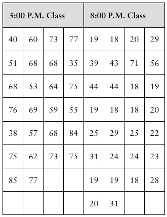
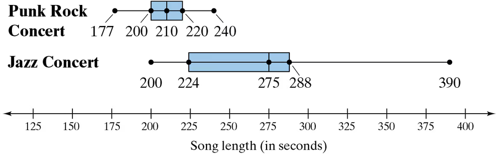
Song Lengths Side-by-side box-and-whisker plots can be used to compare two or more different data sets. Each box-and-whisker plot is drawn on the same number line to compare the data sets more easily. The lengths (in seconds) of songs played at two different concerts are shown.
a. Describe the shape of each distribution. Which concert has less variation in song lengths?
Problem 2.1.45a
What Would You Do? You work at a bank and are asked to recommend the amount of cash to put in an ATM each day. You do not want to put in too much (which would cause security concerns) or too little (which may create customer irritation). The daily withdrawals (in hundreds of dollars) for 30 days are listed. 72 84 61 76 104 76 86 92 80 88 98 76 97 82 84 67 70 81 82 89 74 73 86 81 85 78 82 80 91 83
Construct a relative frequency histogram for the data. Use 8 classes.
Problem 2.3.65a
Extending Concepts
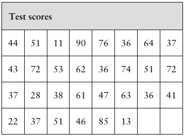
Data Analysis Students in an experimental psychology class did research on depression as a sign of stress. A test was administered to a sample of 30 students. The scores are shown in the table at the left.
a. Find the mean and the median of the data.
Problem 2.4.55a
Pearson’s Index of Skewness The English statistician Karl Pearson (1857–1936) introduced a formula for the skewness of a distribution.
P = 3 (x̄ - median) / s
Most distributions have an index of skewness between -3 and 3. When P > 0, the data are skewed right. When P < 0, the data are skewed left. When P = 0, the data are symmetric. Calculate the coefficient of skewness for each distribution. Describe the shape of each.
a. x̄ = 17, s = 2.3, median = 19
Problem 2.4.11a
Archaeology The depths (in inches) at which 10 artifacts are found are listed.
20.7 24.8 30.5 26.2 36.0 34.3 30.3 29.5 27.0 38.5
a. Find the range of the data set.
Problem 2.2.54a
Shifting Data Sample annual salaries (in thousands of dollars) for employees at a company are listed.
40 35 49 53 38 39 40
37 49 34 38 43 47 35
a. Find the sample mean and the sample standard deviation.
Problem 2.5.17a
Drawing a Box-and-Whisker Plot In Exercises 15–18,
(a) find the five-number summary
4 7 7 5 2 9 7 6 8 5 8 4 1 5 2 8 7 6 6 9
Problem 2.1.19a
Use the frequency histogram
a. to determine the number of classes.
Problem 2.5.16b
Drawing a Box-and-Whisker Plot In Exercises 15–18,
(b) draw a box-and-whisker plot that represents the data set.
171 176 182 150 178 180 173 170 174 178 181 180
Problem 2.3.66b
Extending Concepts
Trimmed Mean To find the 10% trimmed mean of a data set, order the data, delete the lowest 10% of the entries and the highest 10% of the entries, and find the mean of the remaining entries.
b. Compare the four measures of central tendency, including the midrange.
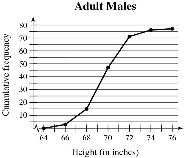
Problem 2.1.28b
Use the ogive to approximate
the height for which the cumulative frequency is 15.
Problem 2.5.17b
Drawing a Box-and-Whisker Plot In Exercises 15–18,
(b) draw a box-and-whisker plot that represents the data set.
4 7 7 5 2 9 7 6 8 5 8 4 1 5 2 8 7 6 6 9
Problem 2.1.45b
What Would You Do? You work at a bank and are asked to recommend the amount of cash to put in an ATM each day. You do not want to put in too much (which would cause security concerns) or too little (which may create customer irritation). The daily withdrawals (in hundreds of dollars) for 30 days are listed. 72 84 61 76 104 76 86 92 80 88 98 76 97 82 84 67 70 81 82 89 74 73 86 81 85 78 82 80 91 83
If you put $9000 in the ATM each day, what percent of the days in a month should you expect to run out of cash? Explain.
Problem 2.4.53b
Scaling Data Sample annual salaries (in thousands of dollars) for employees at a company are listed.
42 36 48 51 39 39 42
36 48 33 39 42 45 50
b. Each employee in the sample receives a 5% raise. Find the sample mean and the sample standard deviation for the revised data set.
Problem 2.5.50b
Life Spans of Fruit Flies The life spans of a species of fruit fly have a bell-shaped distribution, with a mean of 33 days and a standard deviation of 4 days.
b. The life spans of three randomly selected fruit flies are 29 days, 41 days, and 25 days. Using the Empirical Rule, find the percentile that corresponds to each life span.
Problem 2.1.23b
Use the relative frequency histogram to
approximate the greatest and least relative frequencies.
Problem 2.5.18b
Drawing a Box-and-Whisker Plot In Exercises 15–18,
(b) draw a box-and-whisker plot that represents the data set.
2 7 1 3 1 2 8 9 9 2 5 4 7 3 7 5 4
2 3 5 9 5 6 3 9 3 4 9 8 8 2 3 9 5