Back
BackProblem 2.Q.1a
The data set represents the number of minutes a sample of 27 people exercise each week.
108 139 120 123 120 132 123 131 131
157 150 124 111 101 135 119 116 117
127 128 139 119 118 114 127 142 130
a. Construct a frequency distribution for the data set using five classes. Include class limits, midpoints, boundaries, frequencies, relative frequencies, and cumulative frequencies.
Problem 2.Q.1d
The data set represents the number of minutes a sample of 27 people exercise each week.
108 139 120 123 120 132 123 131 131
157 150 124 111 101 135 119 116 117
127 128 139 119 118 114 127 142 130
d. Describe the shape of the distribution as symmetric, uniform, skewed left, skewed right, or none of these.
Problem 2.Q.6d
Refer to the sample statistics from Exercise 5 and determine whether any of the house prices below are unusual. Explain your reasoning.
d. $147,000
Problem 2.Q.4a
Weekly salaries (in dollars) for a sample of construction workers are listed.
1100 720 1384 1124 1255 976 718 1316
749 1062 1248 891 969 790 860 1100
a. Find the mean, median, and mode of the salaries. Which best describes a typical salary?
Problem 2.Q.1b
The data set represents the number of minutes a sample of 27 people exercise each week.
108 139 120 123 120 132 123 131 131
157 150 124 111 101 135 119 116 117
127 128 139 119 118 114 127 142 130
b. Display the data using a frequency histogram and a frequency polygon on the same axes.
Problem 2.Q.1g
The data set represents the number of minutes a sample of 27 people exercise each week.
108 139 120 123 120 132 123 131 131
157 150 124 111 101 135 119 116 117
127 128 139 119 118 114 127 142 130
g. Display the data using a box-and-whisker plot.
Problem 2.R.31
The mean sale per customer for 40 customers at a gas station is $32.00, with a standard deviation of $4.00. Using Chebychev’s Theorem, determine at least how many of the customers spent between $24.00 and $40.00.
Problem 2.R.19
Describe the shape of the distribution for the histogram you made in Exercise 3 as symmetric, uniform, skewed left, skewed right, or none of these.
Problem 2.R.43
A student’s test grade of 75 represents the 65th percentile of the grades. What percent of students scored higher than 75?
Problem 2.R.40
In Exercises 37– 40, use the data set, which represents the model 2020 vehicles with the highest fuel economies (in miles per gallon) in the most popular classes. (Source: U.S. Environmental Protection Agency)
36 30 30 45 31 113 113 33 33 33 52 141 56 117 58
118 50 26 23 23 27 48 22 22 22 121 41 105 35 35
About how many vehicles fall on or below the third quartile?
Problem 2.R.11
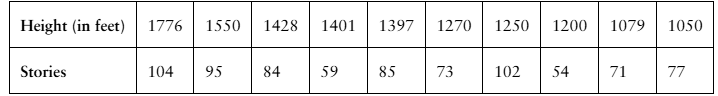
The heights (in feet) and the number of stories of the ten tallest buildings in New York City are listed. Use a scatter plot to display the data. Describe any patterns. (Source: Emporis)
Problem 2.R.34
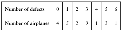
From a random sample of airplanes, the number of defects found in their fuselages are listed. Find the sample mean and the sample standard deviation of the data.
Problem 2.R.8
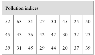
In Exercises 7 and 8, use the data set shown in the table at the left, which represents the pollution indices (a unitless measure of pollution ranging from 0 to 100) for 24 U.S. cities. (Adapted from Numbeo)
Use a dot plot to display the data set. Describe any patterns.
Problem 2.R.17
In Exercises 17–19, use the data set, which represents the points recorded by each player on the Winnipeg Jets in the 2019–2020 NHL season. (Source: National Hockey League)
8 8 8 6 0 73 26 1
0 5 58 1 7 5 10 63
0 5 10 0 31 5 15 45
16 29 10 73 5 3 0 65
Construct a frequency distribution for the data set using eight classes. Include class limits, midpoints, boundaries, frequencies, relative frequencies, and cumulative frequencies.
Problem 2.R.37
In Exercises 37– 40, use the data set, which represents the model 2020 vehicles with the highest fuel economies (in miles per gallon) in the most popular classes. (Source: U.S. Environmental Protection Agency)
36 30 30 45 31 113 113 33 33 33 52 141 56 117 58
118 50 26 23 23 27 48 22 22 22 121 41 105 35 35
Find the five-number summary of the data set.
Problem 2.R.22
In Exercises 21 and 22, determine whether the approximate shape of the distribution in the histogram is symmetric, uniform, skewed left, skewed right, or none of these.
Problem 2.R.46
The towing capacities (in pounds) of all the pickup trucks at a dealership have a bell-shaped distribution, with a mean of 11,830 pounds and a standard deviation of 2370 pounds. In Exercises 45– 48, use the corresponding z-score to determine whether the towing capacity is unusual. Explain your reasoning.
5,500 pounds
Problem 2.R.28
In Exercises 27 and 28, find the range, mean, variance, and standard deviation of the sample data set.
Salaries (in dollars) of a random sample of teachers
62,222 56,719 50,259 45,120 47,692 45,985 53,489 71,534
Problem 2.R.25
In Exercises 25 and 26, find the range, mean, variance, and standard deviation of the population data set.
The mileages (in thousands of miles) for a rental car company’s fleet.
4 2 9 12 15 3 6 8 1 4 14 12 3 3
Problem 2.RE.16
For the four test scores 96, 85, 91, and 86, the first 3 test scores are 20% of the final grade, and the last test score is 40% of the final grade. Find the weighted mean of the test scores.
Problem 2.RE.5
In Exercises 5 and 6, use the data set, which represents the number of rooms reserved during one night’s business at a sample of hotels.
153 104 118 166 89 104 100 79 93 96 116
94 140 84 81 96 108 111 87 126 101 111
122 108 126 93 108 87 103 95 129 93 124
Construct a frequency distribution for the data set with six classes and draw a frequency polygon.
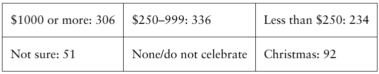
Problem 2.RE.14
In Exercises 13 and 14, find the mean, the median, and the mode of the data, if possible. If any measure cannot be found or does not represent the center of the data, explain why.
The responses of 1019 adults who were asked how much money they think they will spend on Christmas gifts in a recent year (Adapted from Gallup)
Problem 2.RE.2
In Exercises 1 and 2, use the data set, which represents the overall average class sizes for 20 national universities. (Adapted from Public University Honors)
37 34 42 44 39 40 41 51 49 31
52 26 31 40 30 27 36 43 48 35
Construct a relative frequency histogram using the frequency distribution in Exercise 1. Then determine which class has the greatest relative frequency and which has the least relative frequency.
Problem 2.T.1d
The overall averages of 12 students in a statistics class prior to taking the final exam are listed.
67 72 88 73 99 85 81 87 63 94 68 87
d. Display the data in a stem-and-leaf plot. Use one line per stem.
Problem 2.T.1a
The overall averages of 12 students in a statistics class prior to taking the final exam are listed.
67 72 88 73 99 85 81 87 63 94 68 87
a. Find the mean, median, and mode of the data set. Which best represents the center of the data?
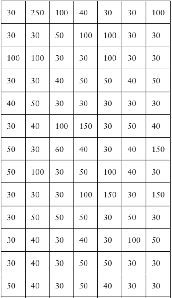
Problem 2.T.5
"According to data from the city of Toronto, Ontario, Canada, there were nearly 112,000 parking infractions in the city for December 2020, with fines totaling over 5,500,000 Canadian dollars. The fines (in Canadian dollars) for a random sample of 105 parking infractions in Toronto, Ontario, Canada, for December 2020 are listed below. (Source: City of Toronto)
In Exercises 1–5, use technology. If possible, print your results.
Draw a histogram for the data. Does the distribution appear to be bell-shaped?"
Problem 2.T.9
Use the frequency distribution in Exercise 4 to estimate the sample mean and sample standard deviation of the data. Do the formulas for grouped data give results that are as accurate as the individual entry formulas? Explain.
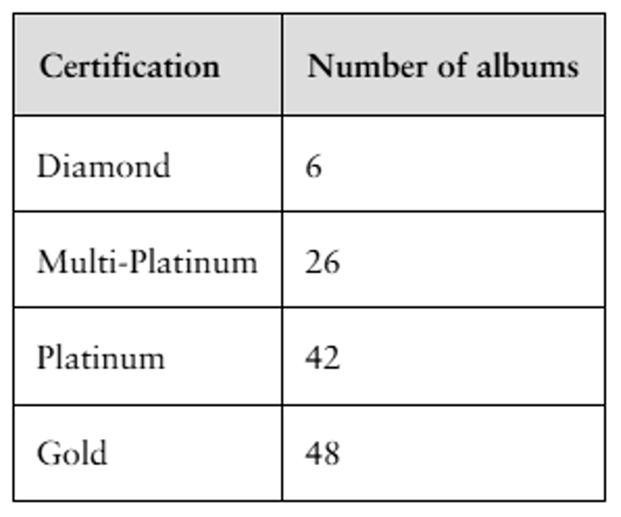
Problem 2.T.5b
The table lists the number of albums by The Beatles that received sales certifications. Display the data using (b) a Pareto chart. (Source: Recording Industry Association of America)
Problem 2.T.8b
The mean gestational length of a sample of 208 horses is 343.7 days, with a standard deviation of 10.4 days. The data set has a bell-shaped distribution.
b. Determine whether a gestational length of 318.4 days is unusual.
Problem 2.T.2c
The data set represents the number of movies that a sample of 20 people watched in a year.
121 148 94 142 170 88 221 106 18 67
149 28 60 101 134 168 92 154 53 66
c. Display the data using a relative frequency histogram.