Back
BackProblem 5.4.8
True or False? In Exercises 5–8, determine whether the statement is true or false. If it is false, rewrite it as a true statement.
If the sample size is at least 30, then you can use z-scores to determine the probability that a sample mean falls in a given interval of the sampling distribution.
Problem 5.2.3
Computing Probabilities for Normal Distributions In Exercises 1–6, the random variable x is normally distributed with mean mu=174 and standard deviation sigma=20. Find the indicated probability.
P(x > 182)
Problem 5.3.21
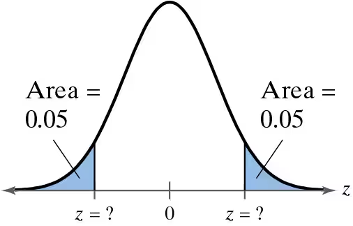
Graphical Analysis In Exercises 17–22, find the indicated z-score(s) shown in the graph.
Problem 5.1.31
Finding Area
In Exercises 23–36, find the indicated area under the standard normal curve. If convenient, use technology to find the area.
Between z=0 and z=2.86
Problem 5.4.1
In Exercises 1– 4, a population has a mean mu and a standard deviation sigma. Find the mean and standard deviation of the sampling distribution of sample means with sample size n.
Mu = 150, sigma =25, n = 49
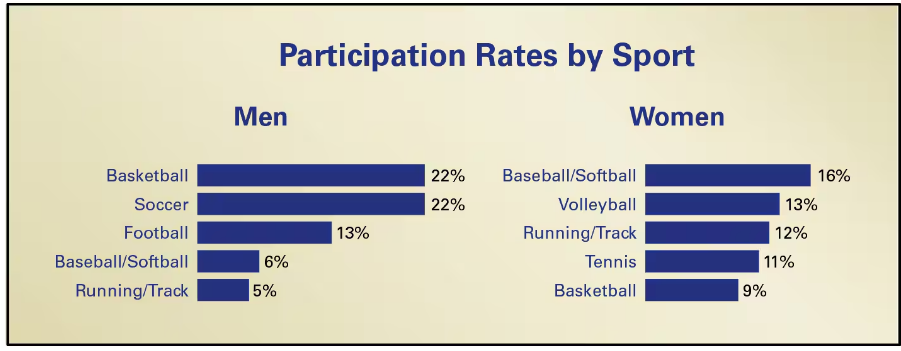
Problem 5.5.30
"Getting Physical The figure shows the results of a survey of U.S. adults ages 18 to 29 who were asked whether they participated in a sport. In the survey, 48% of the men and 23% of the women said they participate in sports. The most common sports are shown below. Use this information in Exercises 29 and 30.
You randomly select 300 U.S. women ages 18 to 29 and ask them whether they participate in at least one sport. Of the 72 who say yes, 50% say they participate in volleyball. How likely is this result? Do you think this sample is a good one? Explain your reasoning."
Problem 5.1.23
Finding Area
In Exercises 23–36, find the indicated area under the standard normal curve. If convenient, use technology to find the area.
To the left of z=0.33
Problem 5.4.26
Interpreting the Central Limit Theorem In Exercises 19–26, find the mean and standard deviation of the indicated sampling distribution of sample means. Then sketch a graph of the sampling distribution.
SAT Italian Subject Test The scores on the SAT Italian Subject Test for the 2018–2020 graduating classes are normally distributed, with a mean of 628 and a standard deviation of 110. Random samples of size 25 are drawn from this population, and the mean of each sample is determined.
Problem 5.1.58
Writing Draw a normal curve with a mean of 450 and a standard deviation of 50. Describe how you constructed the curve and discuss its features.
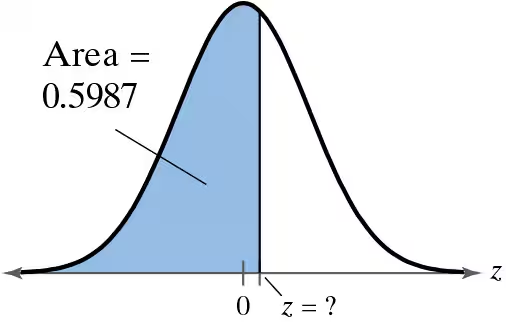
Problem 5.3.18
Graphical Analysis In Exercises 17–22, find the indicated z-score(s) shown in the graph.
Problem 5.5.31
Testing a Drug A drug manufacturer claims that a drug cures a rare skin disease 75% of the time. The claim is checked by testing the drug on 100 patients. If at least 70 patients are cured, then this claim will be accepted. Use this information in Exercises 31 and 32.
Find the probability that the claim will be rejected, assuming that the manufacturer’s claim is true.
Problem 5.3.24
Finding a z-Score Given an Area In Exercises 23–30, find the indicated z-score.
Find the z-score that has 78.5% of the distribution’s area to its left.
Problem 5.4.7
True or False? In Exercises 5–8, determine whether the statement is true or false. If it is false, rewrite it as a true statement.
A sampling distribution is normal only when the population is normal.
Problem 5.4.17
Finding Probabilities In Exercises 15–18, the population mean and standard deviation are given. Find the indicated probability and determine whether the given sample mean would be considered unusual.
For a random sample of n=45, find the probability of a sample mean being greater than 551 when mu=550 and sigma=3.7.
Problem 5.4.20
Interpreting the Central Limit Theorem In Exercises 19–26, find the mean and standard deviation of the indicated sampling distribution of sample means. Then sketch a graph of the sampling distribution.
Renewable Energy The zloty is the official currency of Poland. During a recent period of two years, the day-ahead prices for renewable energy in Poland (in zlotys per mega-watt hour) have a mean of 158.51 and a standard deviation of 33.424. Random samples of size 100 are drawn from this population, and the mean of each sample is determined. (Adapted from Multidisciplinary Digital Publishing Institute)
Problem 5.1.3
Describe the inflection points on the graph of a normal distribution. At what x-values are the inflection points located?
Problem 5.4.3
In Exercises 1– 4, a population has a mean mu and a standard deviation sigma. Find the mean and standard deviation of the sampling distribution of sample means with sample size n.
Mu = 790, sigma =48, n = 250
Problem 5.C.4a
Use the probability distribution in Exercise 3 to find the probability of randomly selecting a game in which DeMar DeRozan had (a) fewer than four personal fouls,
Problem 5.CR.1c
A survey of adults in the United States found that 61% ate at a restaurant at least once in the past week. You randomly select 30 adults and ask them whether they ate at a restaurant at least once in the past week. (Source: Gallup)
c. Is it unusual for exactly 14 out of 30 adults to have eaten in a restaurant at least once in the past week? Explain your reasoning.
Problem 5.CR.6
In Exercises 6–11, find the indicated area under the standard normal curve. If convenient, use technology to find the area.
To the left of z = 0.72
Problem 5.CR.9
In Exercises 6–11, find the indicated area under the standard normal curve. If convenient, use technology to find the area.
Between z = 0 and z = 2.95
Problem 5.CR.12a
Forty-nine percent of U.S. adults think that human activity such as burning fossil fuels contributes a great deal to climate change. You randomly select 25 U.S. adults. Find the probability that the number who think that human activity contributes a great deal to climate change is (a) exactly 12,
Problem 5.CR.4c
Use the probability distribution in Exercise 3 to find the probability of randomly selecting a game in which DeMar DeRozan had (c) between two and four personal fouls, inclusive.
Problem 5.CR.15b
The initial pressures for bicycle tires when first filled are normally distributed, with a mean of 70 pounds per square inch (psi) and a standard deviation of 1.2 psi.
b. A random sample of 15 tires is drawn from this population. What is the probability that the mean tire pressure of the sample is less than 69 psi?
Problem 5.CR.12b
Forty-nine percent of U.S. adults think that human activity such as burning fossil fuels contributes a great deal to climate change. You randomly select 25 U.S. adults. Find the probability that the number who think that human activity contributes a great deal to climate change is (b) between 8 and 11, inclusive,
Problem 5.CR.16c
The life spans of car batteries are normally distributed, with a mean of 44 months and a standard deviation of 5 months.
c. What is the shortest life expectancy a car battery can have and still be in the top 5% of life expectancies?
Problem 5.CR.12c
Forty-nine percent of U.S. adults think that human activity such as burning fossil fuels contributes a great deal to climate change. You randomly select 25 U.S. adults. Find the probability that the number who think that human activity contributes a great deal to climate change is (c) less than two. (d) Are any of these events unusual? Explain your reasoning.
Problem 5.Q.1b
Find each probability using the standard normal distribution.
b. P(z < 2.23)
Problem 5.Q.11
In a survey of U.S. adults, 81% feel they have little or no control over data collected about them by companies. You randomly select 250 U.S. adults and ask them whether they feel they have control over data collected about them by companies. Use this information in Exercises 11 and 12. (Source: Pew Research Center)
Determine whether you can use a normal distribution to approximate the binomial distribution. If you can, find the mean and standard deviation. If you cannot, explain why.
Problem 5.Q.8
In a standardized IQ test, scores are normally distributed, with a mean score of 100 and a standardized deviation of 15. Use this information in Exercises 3–10. (Adapted from 123test)
What is the highest score that would still place a person in the bottom 10% of the scores?