Back
BackProblem 3.2.33
Identifying Significant Values with the Range Rule of Thumb. In Exercises 33–36, use the range rule of thumb to identify the limits separating values that are significantly low or significantly high.
U.S. Presidents Based on Data Set 22 “Presidents” in Appendix B, at the time of their first inauguration, presidents have a mean age of 55.2 years and a standard deviation of 6.9 years. Is the minimum required 35-year age for a president significantly low?
Problem 3.3.23
In Exercises 21–28, use the same list of cell phone radiation levels given for Exercises 17–20. Find the indicated percentile or quartile.
Q3
Problem 3.1.37
Trimmed Mean Because the mean is very sensitive to extreme values, we say that it is not a resistant measure of center. By deleting some low values and high values, the trimmed mean is more resistant. To find the 10% trimmed mean for a data set, first arrange the data in order, then delete the bottom 10% of the values and delete the top 10% of the values, then calculate the mean of the remaining values. Use the axial loads (pounds) of aluminum cans listed below (from Data Set 41 “Aluminum Cans” in Appendix B) for cans that are 0.0111 in. thick. An axial load is the force at which the top of a can collapses. Identify any outliers, then compare the median, mean, 10% trimmed mean, and 20% trimmed mean.
247 260 268 273 276 279 281 283 284 285 286 288
289 291 293 295 296 299 310 504
Problem 3.3.13
Comparing Values. In Exercises 13–16, use z scores to compare the given values.
Tallest and Shortest Men The tallest adult male was Robert Wadlow, and his height was 272 cm. The shortest adult male was Chandra Bahadur Dangi, and his height was 54.6 cm. Heights of men have a mean of 174.12 cm and a standard deviation of 7.10 cm. Which of these two men has the height that is more extreme?
Problem 3.2.5
In Exercises 5–20, find the range, variance, and standard deviation for the given sample data. Include appropriate units (such as “minutes”) in your results. (The same data were used in Section 3-1, where we found measures of center. Here we find measures of variation.) Then answer the given questions.
Super Bowl Jersey Numbers Listed below are the jersey numbers of the 11 offensive players on the starting roster of the New England Patriots when they won Super Bowl LIII. What do the results tell us?
12 26 46 15 11 87 77 62 60 69 61
Problem 3.2.37
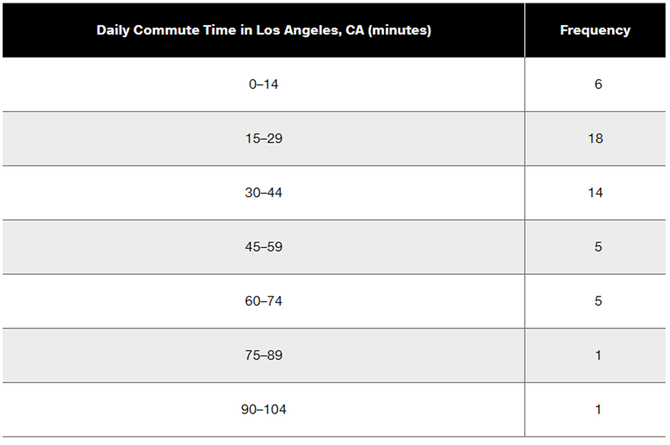
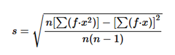
Finding Standard Deviation from a Frequency Distribution. In Exercises 37–40, refer to the frequency distribution in the given exercise and compute the standard deviation by using the formula below, where x represents the class midpoint, f represents the class frequency, and n represents the total number of sample values. Also, compare the computed standard deviations to these standard deviations obtained by using Formula 3-4 with the original list of data values: (Exercise 37) 18.5 minutes; (Exercise 38) 36.7 minutes; (Exercise 39) 6.9 years; (Exercise 40) 20.4 seconds.
Standard deviation for frequency distribution
Problem 3.3.10
Significant Values. In Exercises 9–12, use the range rule of thumb to identify (a) the values that are significantly low, (b) the values that are significantly high, and (c) the values that are neither significantly low nor significantly high.
IQ Scores The Wechsler test is used to measure intelligence of adults aged 16 to 80. The mean test score is 100 and the standard deviation is 15.
Problem 3.3.22
In Exercises 21–28, use the same list of cell phone radiation levels given for Exercises 17–20. Find the indicated percentile or quartile.
Q1
Problem 3.1.11
Critical Thinking. For Exercises 5–20, watch out for these little buggers. Each of these exercises involves some feature that is somewhat tricky. Find the (a) mean, (b) median, (c) mode, (d) midrange, and then answer the given question.
Smart Thermostats Listed below are selling prices (dollars) of smart thermostats tested by Consumer Reports magazine. If you decide to buy one of these smart thermostats, what statistic is most relevant, other than the measures of central tendency?
250 170 225 100 250 250 130 200 150 250 170 200 180 250
Problem 3.1.13
Critical Thinking. For Exercises 5–20, watch out for these little buggers. Each of these exercises involves some feature that is somewhat tricky. Find the (a) mean, (b) median, (c) mode, (d) midrange, and then answer the given question.
Caffeine in Soft Drinks Listed below are measured amounts of caffeine (mg per 12 oz of drink) obtained in one can from each of 20 brands (7-UP, A&W Root Beer, Cherry Coke, . . . , Tab). Are the statistics representative of the population of all cans of the same 20 brands consumed by Americans?
0 0 34 34 34 45 41 51 55 36 47 41 0 0 53 54 38 0 41 47
Problem 3.3.17
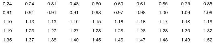
Percentiles. In Exercises 17–20, use the following radiation levels (in W/kg) for 50 different cell phones. Find the percentile corresponding to the given radiation level.
0.48 W/kg
Problem 3.1.21
In Exercises 21–24, find the mean and median for each of the two samples, then compare the two sets of results.
Blood Pressure A sample of blood pressure measurements is taken from Data Set 1 “Body Data” in Appendix B, and those values (mm Hg) are listed below. The values are matched so that 10 subjects each have systolic and diastolic measurements. (Systolic is a measure of the force of blood being pushed through arteries, but diastolic is a measure of blood pressure when the heart is at rest between beats.) Are the measures of center the best statistics to use with these data? What else might be better?
Systolic: 118 128 158 96 156 122 116 136 126 120
Diastolic: 80 76 74 52 90 88 58 64 72 82
Problem 3.3.21
In Exercises 21–28, use the same list of cell phone radiation levels given for Exercises 17–20. Find the indicated percentile or quartile.
P30
Problem 3.1.39
Geometric Mean The geometric mean is often used in business and economics for finding average rates of change, average rates of growth, or average ratios. To find the geometric mean of n values (all of which are positive), first multiply the values, then find the nth root of the product. For a 6-year period, money deposited in annual certificates of deposit had annual interest rates of 0.58%, 0.29%, 0.13%, 0.14%, 0.15%, and 0.19%. Identify the single percentage growth rate that is the same as the six consecutive growth rates by computing the geometric mean of 1.0058, 1.0029, 1.0013, 1.0014, 1.0015, and 1.0019.
Problem 3.3.32
Boxplots. In Exercises 29–32, use the given data to construct a boxplot and identify the 5-number summary.
Blood Pressure Measurements Fourteen different second-year medical students at Bellevue Hospital measured the blood pressure of the same person. The systolic readings (mm Hg) are listed below.
138 130 135 140 120 125 120 130 130 144 143 140 130 150
Problem 3.2.29
Estimating Standard Deviation with the Range Rule of Thumb. In Exercises 29–32, refer to the data in the indicated exercise. After finding the range of the data, use the range rule of thumb to estimate the value of the standard deviation. Compare the result to the standard deviation computed using all of the data.
Body Temperatures Refer to Data Set 5 “Body Temperatures” in Appendix B and use the body temperatures for 12:00 AM on day 2.
Problem 3.1.27
Large Data Sets from Appendix B. In Exercises 25–28, refer to the indicated data set in Appendix B. Use software or a calculator to find the means and medians.
Body Temperatures Refer to Data Set 5 “Body Temperatures” in Appendix B and use the body temperatures for 12:00 AM on day 2. Do the results support or contradict the common belief that the mean body temperature is 98.6oF?
Problem 3.3.18
Percentiles. In Exercises 17–20, use the following radiation levels (in W/kg) for 50 different cell phones. Find the percentile corresponding to the given radiation level.
1.47 W/kg
Problem 3.3.4
z Scores If your score on your next statistics test is converted to a z score, which of these z scores would you prefer: -2.00, -1.00, 0, 1.00, 2.00? Why?
Problem 3.3.30
Boxplots. In Exercises 29–32, use the given data to construct a boxplot and identify the 5-number summary.
Taxis Listed below are times (minutes) of a sample of taxi rides in New York City. The data are from the New York City Taxi and Limousine Commission.
15 12 31 3 11 33 62 4
Problem 3.1.8
Critical Thinking. For Exercises 5–20, watch out for these little buggers. Each of these exercises involves some feature that is somewhat tricky. Find the (a) mean, (b) median, (c) mode, (d) midrange, and then answer the given question.
Geography Majors The data listed below are estimated incomes (dollars) of students who graduated from the University of North Carolina (UNC) after majoring in geography. The data are based on graduates in the year 1984. The income of basketball superstar Michael Jordan (a 1984 UNC graduate and geography major) is included. Does his income have much of an effect on the measures of center? Based on these data, would the college have been justified by saying that the mean income of a graduate in their geography program is greater than $250,000?
17,466 18,085 17,875 19,339 19,682 19,610 18,259 16,354 2,200,000
Problem 3.3.33
Boxplots from Large Data Sets in Appendix B. In Exercises 33–36, use the given data sets in Appendix B. Use the boxplots to compare the two data sets.
Pulse Rates Use the same scale to construct boxplots for the pulse rates of males and females from Data Set 1 “Body Data” in Appendix B.
Problem 3.2.9
In Exercises 5–20, find the range, variance, and standard deviation for the given sample data. Include appropriate units (such as “minutes”) in your results. (The same data were used in Section 3-1, where we found measures of center. Here we find measures of variation.) Then answer the given questions.
Jaws 3 Listed below are the number of unprovoked shark attacks worldwide for the last several years. What extremely important characteristic of the data is not considered when finding the measures of variation?
70 54 68 82 79 83 76 73 98 81
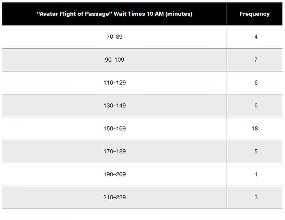
Problem 3.1.24
In Exercises 21–24, find the mean and median for each of the two samples, then compare the two sets of results.
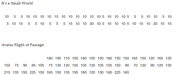
It’s a Small Wait After All Listed below are the wait times (minutes) at 10 AM for the rides “It’s a Small World” and “Avatar Flight of Passage.” These data are found in Data Set 33 “Disney World Wait Times.” Does a comparison between the means and medians reveal that there is a difference between the two sets of data?
Problem 3.1.2
What’s Wrong? Education Week magazine published a list consisting of the mean teacher salary in each of the 50 states for a recent year. If we add the 50 means and then divide by 50, we get $56,479. Is the value of $56,479 the mean teacher salary for the population of all teachers in the 50 United States? Why or why not?
Problem 3.2.6
In Exercises 5–20, find the range, variance, and standard deviation for the given sample data. Include appropriate units (such as “minutes”) in your results. (The same data were used in Section 3-1, where we found measures of center. Here we find measures of variation.) Then answer the given questions.
Super Bowl Ages Listed below are the ages of the same 11 players used in the preceding exercise. How are the resulting statistics fundamentally different from those found in the preceding exercise?
41 24 30 31 32 29 25 26 26 25 30
Problem 3.2.45
Why Divide by ? Let a population consist of the values 9 cigarettes, 10 cigarettes, and 20 cigarettes smoked in a day (based on data from the California Health Interview Survey). Assume that samples of two values are randomly selected with replacement from this population. (That is, a selected value is replaced before the second selection is made.)
a. Find the variance of the population {9 cigarettes, 10 cigarettes, 20 cigarettes}.
Problem 3.2.38
Finding Standard Deviation from a Frequency Distribution. In Exercises 37–40, refer to the frequency distribution in the given exercise and compute the standard deviation by using the formula below, where x represents the class midpoint, f represents the class frequency, and n represents the total number of sample values. Also, compare the computed standard deviations to these standard deviations obtained by using Formula 3-4 with the original list of data values: (Exercise 37) 18.5 minutes; (Exercise 38) 36.7 minutes; (Exercise 39) 6.9 years; (Exercise 40) 20.4 seconds.
Standard deviation for frequency distribution
Problem 3.2.46
Mean Absolute Deviation Use the same population of {9 cigarettes, 10 cigarettes, 20 cigarettes} from Exercise 45. Show that when samples of size 2 are randomly selected with replacement, the samples have mean absolute deviations that do not center about the value of the mean absolute deviation of the population. What does this indicate about a sample mean absolute deviation being used as an estimator of the mean absolute deviation of a population?
Problem 3.1.40
Quadratic Mean The quadratic mean (or root mean square, or R.M.S.) is used in physical applications, such as power distribution systems. The quadratic mean of a set of values is obtained by squaring each value, adding those squares, dividing the sum by the number of values n, and then taking the square root of that result, as indicated below:
Quadratic mean = sqrt(∑x^2/n)
Find the R.M.S. of these voltages measured from household current: 0, 60, 110, 0. How does the result compare to the mean?