Roller Coaster z Score A larger sample of 92 roller coaster maximum speeds has a mean of 85.9 km/h and a standard deviation of 28.7 km/h. What is the z score for a speed of 34 km/h? Does the z score suggest that the speed of 34 km/h is significantly low?

Estimating s The sample of 92 roller coaster maximum speeds includes values ranging from a low of 10 km/h to a high of 194 km/h. Use the range rule of thumb to estimate the standard deviation.

Outliers Identify any of the differences found from Exercise 1 that appear to be outliers. For any outliers, how much of an effect do they have on the mean, median, and standard deviation?

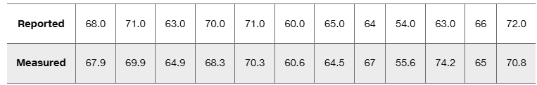
Reported and Measured Heights Listed below are self-reported heights of males aged 16 and over and their corresponding measured heights (based on data from the National Health and Nutrition Examination Survey). All heights are in inches. First find the differences (reported height–measured height), and then use those differences to find the (a) mean, (b) median, (c) mode,

Reported and Measured Heights Listed below are self-reported heights of males aged 16 and over and their corresponding measured heights (based on data from the National Health and Nutrition Examination Survey). All heights are in inches. First find the differences (reported height–measured height), and then use those differences to find the (h) Q1, (i) Q3

Estimating Standard Deviation Listed below are sorted weights (g) of a sample of M&M plain candies randomly selected from one bag. Use the range rule of thumb to estimate the value of the standard deviation of all 345 M&Ms in the bag. Compare the result to the standard deviation of 0.0366 g computed from all of the 345 M&Ms in the bag.

Percentile Use the weights from Exercise 1 to find the percentile for 3647 mg.

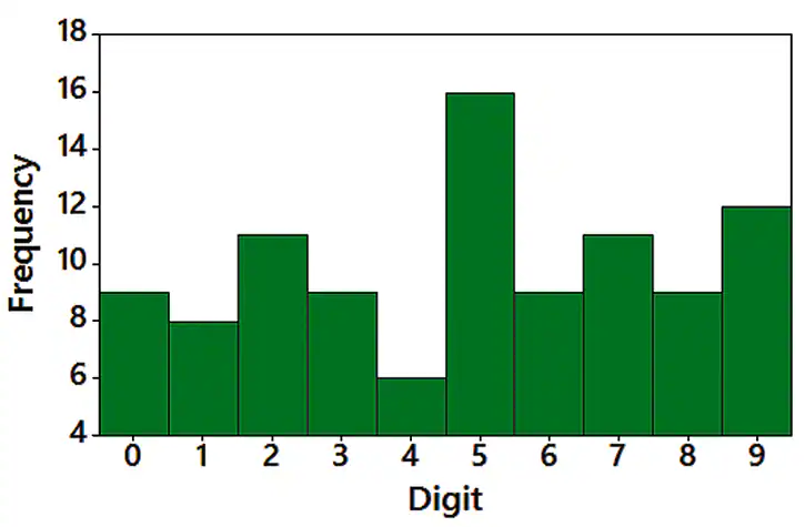
Normal Distribution Examine the distribution shown in the histogram from Exercise 6. Does it appear that the sample data are from a population with a normal distribution? Why or why not?

Geometric Mean The geometric mean is often used in business and economics for finding average rates of change, average rates of growth, or average ratios. To find the geometric mean of n values (all of which are positive), first multiply the values, then find the nth root of the product. For a 6-year period, money deposited in annual certificates of deposit had annual interest rates of 0.58%, 0.29%, 0.13%, 0.14%, 0.15%, and 0.19%. Identify the single percentage growth rate that is the same as the six consecutive growth rates by computing the geometric mean of 1.0058, 1.0029, 1.0013, 1.0014, 1.0015, and 1.0019.

What’s Wrong? Education Week magazine published a list consisting of the mean teacher salary in each of the 50 states for a recent year. If we add the 50 means and then divide by 50, we get $56,479. Is the value of $56,479 the mean teacher salary for the population of all teachers in the 50 United States? Why or why not?

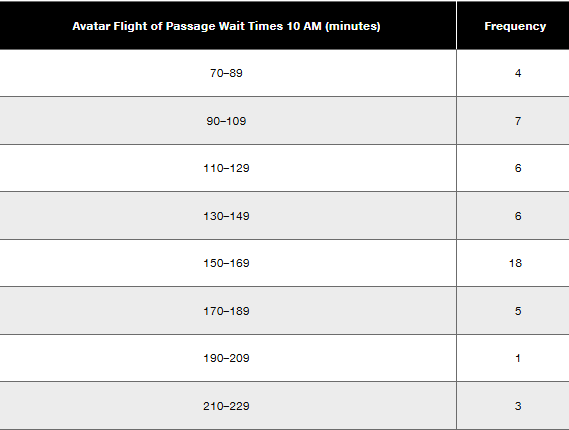
In Exercises 29–32, compute the mean of the data summarized in the frequency distribution. Also, compare the computed means to the actual means obtained by using the original list of data values, which are as follows: (29) 31.4 minutes; (Exercise 30) 140.6 minutes; (Exercise 31) 55.2 years; (Exercise 32) 240.2 seconds.

Weighted Mean A student of the author earned grades of 63, 91, 88, 84, and 79 on her five regular statistics tests. She earned grades of 86 on the final exam and 90 on her class projects. Her combined homework grade was 70. The five regular tests count for 60% of the final grade, the final exam counts for 10%, the project counts for 15%, and homework counts for 15%. What is her weighted mean grade? What letter grade did she earn (A, B, C, D, or F)? Assume that a mean of 90 or above is an A, a mean of 80 to 89 is a B, and so on.

Degrees of Freedom Five recent U.S. presidents had a mean age of 56.2 years at the time of their inauguration. Four of these ages are 64, 46, 54, and 47.

a. Find the missing value.

Trimmed Mean Because the mean is very sensitive to extreme values, we say that it is not a resistant measure of center. By deleting some low values and high values, the trimmed mean is more resistant. To find the 10% trimmed mean for a data set, first arrange the data in order, then delete the bottom 10% of the values and delete the top 10% of the values, then calculate the mean of the remaining values. Use the axial loads (pounds) of aluminum cans listed below (from Data Set 41 “Aluminum Cans” in Appendix B) for cans that are 0.0111 in. thick. An axial load is the force at which the top of a can collapses. Identify any outliers, then compare the median, mean, 10% trimmed mean, and 20% trimmed mean.

247 260 268 273 276 279 281 283 284 285 286 288

289 291 293 295 296 299 310 504

Resistant Measures Listed below are 10 wait times (minutes) for “Rock ‘n’ Roller Coaster” at 10 AM (from Data Set 33 “Disney World Wait Times”). The data are listed in order from lowest to highest. Find the mean and median of these ten values. Then find the mean and median after excluding the value of 180, which appears to be an outlier. Compare the two sets of results. How much was the mean affected by the inclusion of the outlier? How much is the median affected by the inclusion of the outlier?

15 20 25 30 30 35 45 50 50 180 

Critical Thinking. For Exercises 5–20, watch out for these little buggers. Each of these exercises involves some feature that is somewhat tricky. Find the (a) mean, (b) median, (c) mode, (d) midrange, and then answer the given question.

Geography Majors The data listed below are estimated incomes (dollars) of students who graduated from the University of North Carolina (UNC) after majoring in geography. The data are based on graduates in the year 1984. The income of basketball superstar Michael Jordan (a 1984 UNC graduate and geography major) is included. Does his income have much of an effect on the measures of center? Based on these data, would the college have been justified by saying that the mean income of a graduate in their geography program is greater than $250,000?

17,466 18,085 17,875 19,339 19,682 19,610 18,259 16,354 2,200,000

Critical Thinking. For Exercises 5–20, watch out for these little buggers. Each of these exercises involves some feature that is somewhat tricky. Find the (a) mean, (b) median, (c) mode, (d) midrange, and then answer the given question.

Smart Thermostats Listed below are selling prices (dollars) of smart thermostats tested by Consumer Reports magazine. If you decide to buy one of these smart thermostats, what statistic is most relevant, other than the measures of central tendency?

250 170 225 100 250 250 130 200 150 250 170 200 180 250

Critical Thinking. For Exercises 5–20, watch out for these little buggers. Each of these exercises involves some feature that is somewhat tricky. Find the (a) mean, (b) median, (c) mode, (d) midrange, and then answer the given question.

Caffeine in Soft Drinks Listed below are measured amounts of caffeine (mg per 12 oz of drink) obtained in one can from each of 20 brands (7-UP, A&W Root Beer, Cherry Coke, . . . , Tab). Are the statistics representative of the population of all cans of the same 20 brands consumed by Americans?

0 0 34 34 34 45 41 51 55 36 47 41 0 0 53 54 38 0 41 47

In Exercises 21–24, find the mean and median for each of the two samples, then compare the two sets of results.

Blood Pressure A sample of blood pressure measurements is taken from Data Set 1 “Body Data” in Appendix B, and those values (mm Hg) are listed below. The values are matched so that 10 subjects each have systolic and diastolic measurements. (Systolic is a measure of the force of blood being pushed through arteries, but diastolic is a measure of blood pressure when the heart is at rest between beats.) Are the measures of center the best statistics to use with these data? What else might be better?

Systolic: 118 128 158 96 156 122 116 136 126 120

Diastolic: 80  76  74  52  90  88  58   64  72  82

Quadratic Mean The quadratic mean (or root mean square, or R.M.S.) is used in physical applications, such as power distribution systems. The quadratic mean of a set of values is obtained by squaring each value, adding those squares, dividing the sum by the number of values n, and then taking the square root of that result, as indicated below:

Quadratic mean = sqrt(∑x^2/n)

Find the R.M.S. of these voltages measured from household current: 0, 60, 110, 0. How does the result compare to the mean?

Large Data Sets from Appendix B. In Exercises 25–28, refer to the indicated data set in Appendix B. Use software or a calculator to find the means and medians.

Weights Use the weights of the males listed in Data Set 2 “ANSUR I 1988,” which were measured in 1988 and use the weights of the males listed in Data Set 3 “ANSUR II 2012,” which were measured in 2012. Does it appear that males have become heavier?

In Exercises 21–24, find the mean and median for each of the two samples, then compare the two sets of results.

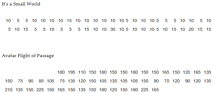
It’s a Small Wait After All Listed below are the wait times (minutes) at 10 AM for the rides “It’s a Small World” and “Avatar Flight of Passage.” These data are found in Data Set 33 “Disney World Wait Times.” Does a comparison between the means and medians reveal that there is a difference between the two sets of data?

Large Data Sets from Appendix B. In Exercises 25–28, refer to the indicated data set in Appendix B. Use software or a calculator to find the means and medians.

Body Temperatures Refer to Data Set 5 “Body Temperatures” in Appendix B and use the body temperatures for 12:00 AM on day 2. Do the results support or contradict the common belief that the mean body temperature is 98.6oF?

In Exercises 5–20, find the range, variance, and standard deviation for the given sample data. Include appropriate units (such as “minutes”) in your results. (The same data were used in Section 3-1, where we found measures of center. Here we find measures of variation.) Then answer the given questions.

Super Bowl Jersey Numbers Listed below are the jersey numbers of the 11 offensive players on the starting roster of the New England Patriots when they won Super Bowl LIII. What do the results tell us?

12 26 46 15 11 87 77 62 60 69 61

In Exercises 5–20, find the range, variance, and standard deviation for the given sample data. Include appropriate units (such as “minutes”) in your results. (The same data were used in Section 3-1, where we found measures of center. Here we find measures of variation.) Then answer the given questions.

Super Bowl Ages Listed below are the ages of the same 11 players used in the preceding exercise. How are the resulting statistics fundamentally different from those found in the preceding exercise?

41 24 30 31 32 29 25 26 26 25 30

Identifying Significant Values with the Range Rule of Thumb. In Exercises 33–36, use the range rule of thumb to identify the limits separating values that are significantly low or significantly high.

Foot Lengths Based on Data Set 9 “Foot and Height” in Appendix B, adult males have foot lengths with a mean of 27.32 cm and a standard deviation of 1.29 cm. Is the adult male foot length of 30 cm significantly low, significantly high, or neither? Explain.

Identifying Significant Values with the Range Rule of Thumb. In Exercises 33–36, use the range rule of thumb to identify the limits separating values that are significantly low or significantly high.

U.S. Presidents Based on Data Set 22 “Presidents” in Appendix B, at the time of their first inauguration, presidents have a mean age of 55.2 years and a standard deviation of 6.9 years. Is the minimum required 35-year age for a president significantly low?

Estimating Standard Deviation with the Range Rule of Thumb. In Exercises 29–32, refer to the data in the indicated exercise. After finding the range of the data, use the range rule of thumb to estimate the value of the standard deviation. Compare the result to the standard deviation computed using all of the data.

Audiometry Use the hearing measurements from Data Set 7 “Audiometry.” Does it appear that the amounts of variation are different for the right threshold measurements and the left threshold measurements?

In Exercises 5–20, find the range, variance, and standard deviation for the given sample data. Include appropriate units (such as “minutes”) in your results. (The same data were used in Section 3-1, where we found measures of center. Here we find measures of variation.) Then answer the given questions.

Jaws 3 Listed below are the number of unprovoked shark attacks worldwide for the last several years. What extremely important characteristic of the data is not considered when finding the measures of variation?

70 54 68 82 79 83 76 73 98 81

In Exercises 5–20, find the range, variance, and standard deviation for the given sample data. Include appropriate units (such as “minutes”) in your results. (The same data were used in Section 3-1, where we found measures of center. Here we find measures of variation.) Then answer the given questions.

Smart Thermostats Listed below are selling prices (dollars) of smart thermostats tested by Consumer Reports magazine. Are any of the resulting statistics helpful in selecting a smart thermostat for purchase?

250 170 225 100 250 250 130 200 150 250 170 200 180 250