Robust Explain what is meant by the statements that the t test for a claim about μ is robust, but the (chi)^2 test for a claim about σ is not robust.
Table of contents
- 1. Intro to Stats and Collecting Data1h 14m
- 2. Describing Data with Tables and Graphs1h 56m
- 3. Describing Data Numerically2h 5m
- 4. Probability2h 16m
- 5. Binomial Distribution & Discrete Random Variables3h 6m
- 6. Normal Distribution and Continuous Random Variables2h 11m
- 7. Sampling Distributions & Confidence Intervals: Mean3h 23m
- Sampling Distribution of the Sample Mean and Central Limit Theorem19m
- Distribution of Sample Mean - Excel23m
- Introduction to Confidence Intervals15m
- Confidence Intervals for Population Mean1h 18m
- Determining the Minimum Sample Size Required12m
- Finding Probabilities and T Critical Values - Excel28m
- Confidence Intervals for Population Means - Excel25m
- 8. Sampling Distributions & Confidence Intervals: Proportion2h 10m
- 9. Hypothesis Testing for One Sample5h 8m
- Steps in Hypothesis Testing1h 6m
- Performing Hypothesis Tests: Means1h 4m
- Hypothesis Testing: Means - Excel42m
- Performing Hypothesis Tests: Proportions37m
- Hypothesis Testing: Proportions - Excel27m
- Performing Hypothesis Tests: Variance12m
- Critical Values and Rejection Regions28m
- Link Between Confidence Intervals and Hypothesis Testing12m
- Type I & Type II Errors16m
- 10. Hypothesis Testing for Two Samples5h 37m
- Two Proportions1h 13m
- Two Proportions Hypothesis Test - Excel28m
- Two Means - Unknown, Unequal Variance1h 3m
- Two Means - Unknown Variances Hypothesis Test - Excel12m
- Two Means - Unknown, Equal Variance15m
- Two Means - Unknown, Equal Variances Hypothesis Test - Excel9m
- Two Means - Known Variance12m
- Two Means - Sigma Known Hypothesis Test - Excel21m
- Two Means - Matched Pairs (Dependent Samples)42m
- Matched Pairs Hypothesis Test - Excel12m
- Two Variances and F Distribution29m
- Two Variances - Graphing Calculator16m
- 11. Correlation1h 24m
- 12. Regression3h 33m
- Linear Regression & Least Squares Method26m
- Residuals12m
- Coefficient of Determination12m
- Regression Line Equation and Coefficient of Determination - Excel8m
- Finding Residuals and Creating Residual Plots - Excel11m
- Inferences for Slope31m
- Enabling Data Analysis Toolpak1m
- Regression Readout of the Data Analysis Toolpak - Excel21m
- Prediction Intervals13m
- Prediction Intervals - Excel19m
- Multiple Regression - Excel29m
- Quadratic Regression15m
- Quadratic Regression - Excel10m
- 13. Chi-Square Tests & Goodness of Fit2h 21m
- 14. ANOVA2h 28m
9. Hypothesis Testing for One Sample
Steps in Hypothesis Testing
Problem 9.3.7a
Textbook Question
In Exercises 5–16, use the listed paired sample data, and assume that the samples are simple random samples and that the differences have a distribution that is approximately normal.
The Freshman 15 The “Freshman 15” refers to the belief that college students gain 15 lb (or 6.8 kg) during their freshman year. Listed below are weights (kg) of randomly selected male college freshmen (from Data Set 13 “Freshman 15” in Appendix B). The weights were measured in September and later in April.
a. Use a 0.01 significance level to test the claim that for the population of freshman male college students, the weights in September are less than the weights in the following April.

 Verified step by step guidance
1
Step 1: Define the null hypothesis (H₀) and the alternative hypothesis (H₁). The null hypothesis is H₀: μ₁ = μ₂, which states that the mean weight in September is equal to the mean weight in April. The alternative hypothesis is H₁: μ₁ < μ₂, which states that the mean weight in September is less than the mean weight in April.
Step 2: Calculate the differences between the paired weights (April - September) for each student. For example, for the first student, the difference is 67 - 67 = 0. Repeat this for all pairs to create a list of differences.
Step 3: Compute the mean (d̄) and standard deviation (s_d) of the differences. Use the formulas: d̄ = (Σd) / n and s_d = sqrt((Σ(d - d̄)²) / (n - 1)), where d represents the differences and n is the number of pairs.
Step 4: Perform a t-test for paired samples. Calculate the test statistic t using the formula: t = (d̄ - 0) / (s_d / sqrt(n)), where 0 is the hypothesized mean difference under H₀. Determine the degrees of freedom (df = n - 1).
Step 5: Compare the calculated t-value to the critical t-value at a significance level of 0.01 and df = n - 1. If the calculated t-value is less than the critical t-value, reject H₀ and conclude that the mean weight in September is less than the mean weight in April. Otherwise, fail to reject H₀.
 Verified video answer for a similar problem:
This video solution was recommended by our tutors as helpful for the problem above
Video duration:
8mPlay a video:
0 Comments
Key Concepts
Here are the essential concepts you must grasp in order to answer the question correctly.
Paired Sample T-Test
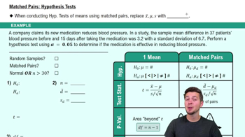
A paired sample t-test is a statistical method used to compare the means of two related groups. In this context, it assesses whether the average weight of male college freshmen in September is significantly less than in April. This test accounts for the fact that the samples are related, as they consist of the same individuals measured at two different times.
Recommended video:
Guided course

Matched Pairs: Hypothesis Tests
Significance Level (α)
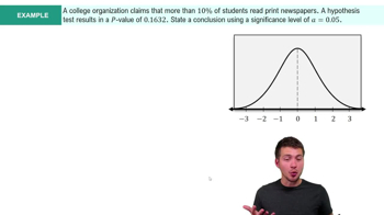
The significance level, denoted as α, is the threshold for determining whether a result is statistically significant. In this case, a significance level of 0.01 indicates that there is a 1% risk of concluding that a difference exists when there is none. This stringent level is often used in studies where the consequences of a Type I error (false positive) are particularly serious.
Recommended video:
Guided course

Step 4: State Conclusion Example 4
Normal Distribution
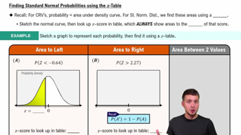
Normal distribution is a probability distribution that is symmetric about the mean, indicating that data near the mean are more frequent in occurrence than data far from the mean. The assumption of normality is crucial for the validity of the paired sample t-test, as it ensures that the test statistics follow a predictable distribution under the null hypothesis.
Recommended video:
Guided course

Finding Standard Normal Probabilities using z-Table

 6:21m
6:21mWatch next
Master Step 1: Write Hypotheses with a bite sized video explanation from Patrick
Start learningRelated Videos
Related Practice
Textbook Question
