Frequency Distributions: Videos & Practice Problems

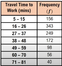
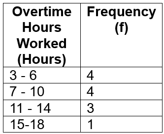
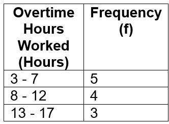
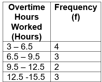
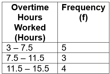
Understanding how to visualize data effectively is crucial in data analysis, and one of the foundational tools for this is the frequency distribution. A frequency distribution is essentially a table that organizes data into classes, showing how many measurements fall into each category. This method is particularly useful for both qualitative and quantitative data, allowing for a clearer interpretation of the information.

To construct a frequency distribution, you first need to define your classes, which are the ranges of values that group your data. For example, if you have a dataset representing the time students spend studying, you might create classes such as 20-29 minutes, 30-39 minutes, and so on. In this case, you would identify how many data points fall into each class, which is referred to as the frequency.

To illustrate, if you have a dataset ranging from 20 to 75 minutes, you would count how many values fall within each defined class. For instance, if you find that there is 1 student studying between 20-29 minutes, 2 students between 30-39 minutes, and so forth, you would record these counts in your frequency distribution table.

Key terms to understand in this context include:

• Lower Class Limit: The smallest value in each class. For example, in the class 20-29, the lower class limit is 20.
• Upper Class Limit: The largest value in each class. For the class 20-29, the upper class limit is 29.
• Class Midpoint: The average of the lower and upper limits of a class, calculated as \( \text{Midpoint} = \frac{\text{Lower Limit} + \text{Upper Limit}}{2} \). For the class 20-29, the midpoint would be \( \frac{20 + 29}{2} = 24.5 \).
• Class Width: The difference between the lower limits of consecutive classes. For example, the class width between 20-29 and 30-39 is \( 30 - 20 = 10 \).

Once you have established the frequency distribution, you may also want to calculate the relative frequency, which expresses the frequency of each class as a percentage of the total number of observations. This is done using the formula:

Relative Frequency = \( \frac{f}{n} \times 100 \)

where \( f \) is the frequency of the class and \( n \) is the total number of observations. For instance, if the total number of students is 10, and there is 1 student in the 20-29 class, the relative frequency would be \( \frac{1}{10} \times 100 = 10\% \).

By organizing data into a frequency distribution and calculating relative frequencies, you can gain valuable insights into the distribution of your data, making it easier to visualize and analyze trends.

In this example, we explore how to create a frequency distribution based on customer counts at a cafe over a 14-hour period. We start with a lower class limit of 15 and a class width of 5, which helps us define our classes. The classes are determined as follows: the first class is 15-19, the second is 20-24, and this continues up to 40-44. However, since the highest customer count is 41, we stop at the class 40-44, as it contains no data values.

Next, we identify the upper class limits by subtracting 1 from each lower class limit. This gives us the upper limits of 19, 24, 29, 34, 39, and 44. With our classes established, we can now tally the number of customers that fall into each class. By counting the data values, we find the frequencies: 1 for 15-19, 2 for 20-24, 4 for 25-29, 3 for 30-34, 2 for 35-39, and 2 for 40-44. Adding these frequencies confirms a total of 14 customers.

To further analyze the data, we calculate the relative frequencies, which represent the proportion of each class relative to the total number of observations. The formula for relative frequency is given by:

$\frac{f}{n}100$

where f is the frequency of the class and n is the total number of observations (14 in this case). For example, the relative frequency for the first class (15-19) is calculated as:

$\frac{1}{14}=0.071$

Continuing this process for each class yields relative frequencies of 0.14 for the second and third classes, 0.28 for the fourth class, and 0.21 for the fifth class. The last class also has a relative frequency of 0.14.

Finally, we address the question of what percentage of the time the cafe serves 30 or more customers per hour. This involves summing the relative frequencies of the classes that represent 30 customers and above, which are the classes 30-34, 35-39, and 40-44. Adding these relative frequencies (0.28 + 0.21 + 0.14) results in 0.63. Converting this decimal to a percentage gives us 63%. Thus, 63% of the time, the cafe serves 30 or more customers per hour.

Frequency distributions are essential tools for organizing data into classes, allowing for easier analysis of the frequency of occurrences within specified ranges. When constructing a frequency distribution, particularly when only the number of classes is provided, a systematic approach is necessary to determine the class limits and widths.

The first step in this process is to calculate the class width. This is done by taking the difference between the maximum and minimum values of the dataset and dividing it by the number of classes. The formula for class width can be expressed as:

$$ \text{Class Width} = \frac{\text{Maximum} - \text{Minimum}}{\text{Number of Classes}} $$

For example, if the maximum value is 115 and the minimum is 5, the calculation would be:

$$ \text{Class Width} = \frac{115 - 5}{8} = \frac{110}{8} = 13.75 $$

Since class widths are typically rounded to a convenient number, you might choose to round 13.75 up to 14 or 15, depending on the context. In this case, using 15 as the class width simplifies the calculations.

Next, you need to determine the lower class limits. The first lower class limit is often set at or below the minimum value of the dataset. In this example, using 5 as the first lower limit is appropriate. Subsequent lower class limits are found by adding the class width to the previous lower limit:

1. First lower limit: 5

2. Second lower limit: 5 + 15 = 20

3. Third lower limit: 20 + 15 = 35

4. Fourth lower limit: 35 + 15 = 50

5. Fifth lower limit: 50 + 15 = 65

6. Sixth lower limit: 65 + 15 = 80

7. Seventh lower limit: 80 + 15 = 95

8. Eighth lower limit: 95 + 15 = 110

Now, to find the upper class limits, take the second lower limit and subtract 1. This prevents double counting of data values that fall on the boundary between two classes:

1. First upper limit: 20 - 1 = 19

2. Second upper limit: 35 - 1 = 34

3. Third upper limit: 50 - 1 = 49

4. Fourth upper limit: 65 - 1 = 64

5. Fifth upper limit: 80 - 1 = 79

6. Sixth upper limit: 95 - 1 = 94

7. Seventh upper limit: 110 - 1 = 109

8. Eighth upper limit: 125 - 1 = 124

With the lower and upper class limits established, you can now tally the frequencies for each class by counting how many data points fall within each range. For instance:

• 5 to 19: 2
• 20 to 34: 2
• 35 to 49: 4
• 50 to 64: 6
• 65 to 79: 2
• 80 to 94: 2
• 95 to 109: 1
• 110 to 124: 1

Thus, the final frequency distribution for the dataset is summarized as follows:

• 5-19: 2
• 20-34: 2
• 35-49: 4
• 50-64: 6
• 65-79: 2
• 80-94: 2
• 95-109: 1
• 110-124: 1

Understanding how to create frequency distributions from raw data is a valuable skill in data analysis, enabling clearer insights into patterns and trends within the dataset.

In constructing a frequency distribution for a dataset representing the sales in dollars of 15 sales representatives, the first step is to determine the class width. This is calculated by taking the maximum value from the dataset, subtracting the minimum value, and then dividing by the number of classes. In this case, the maximum sales figure is 1223, and the minimum is 819. The formula for class width (CW) can be expressed as:

$$ CW = \frac{Max - Min}{Number \ of \ Classes} $$

Substituting the values, we have:

$$ CW = \frac{1223 - 819}{5} = \frac{404}{5} = 80.8 $$

Since class widths are typically rounded to whole numbers for practical purposes, we round 80.8 up to 81. This means that each class will span 81 units.

Next, we establish the lower class limits. The first lower class limit is set at the minimum value of the dataset, which is 819. Each subsequent lower class limit is determined by adding the class width to the previous lower limit:

1. 819 (first lower limit)

2. 900 (819 + 81)

3. 981 (900 + 81)

4. 1062 (981 + 81)

5. 1143 (1062 + 81)

6. 1224 (1143 + 81, but this exceeds the maximum value)

For the upper class limits, each upper limit is found by subtracting 1 from the next lower limit:

1. 899 (900 - 1)

2. 980 (981 - 1)

3. 1061 (1062 - 1)

4. 1142 (1143 - 1)

5. 1223 (1224 - 1)

With the lower and upper class limits established, we can now tally the frequencies of the sales figures that fall within each class. By analyzing the dataset, we categorize each sales figure into its respective class and count the occurrences:

- For the class 819 to 899, we find 1 occurrence.

- For the class 900 to 980, we find 4 occurrences.

- For the class 981 to 1061, we find 5 occurrences.

- For the class 1062 to 1142, we find 2 occurrences.

- For the class 1143 to 1223, we find 3 occurrences.

Summing these frequencies confirms that all 15 sales figures have been accounted for, resulting in a complete frequency distribution:

This frequency distribution effectively summarizes the sales data, allowing for easier analysis and interpretation of the sales performance of the representatives.