Back
BackProblem 9.3.10
"In Exercises 7-10, use the value of the correlation coefficient r to calculate the coefficient of determination r^2. What does this tell you about the explained variation of the data about the regression line? about the unexplained variation?
10. r =0.881"
Problem 9.1.32
In Exercise 26, add data for an international soccer player who can perform the half squat with a maximum of 210 kilograms and can sprint 10 meters in 2.00 seconds. Describe how this affects the correlation coefficient r.
Problem 9.Q.8
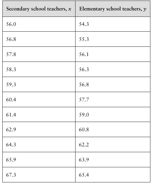
"[APPLET] For Exercises 1– 8, use the data in the table, which shows the average annual salaries (both in thousands of dollars) for secondary and elementary school teachers, excluding special and vocational education teachers, in the United States for 11 years. (Source: U.S. Bureau of Labor Statistics)
8. Construct a 95% prediction interval for the average annual salary of elementary school teachers when the average annual salary of secondary school teachers is $63,500. Interpret the results."
Problem 9.Q.9
"9. Stock Price The equation used to predict the stock price (in dollars) at the end of the year for a restaurant chain is y=- 86+7.46x_1 - 1.61x_2
where x_1 is the total revenue (in billions of dollars) and x_2 is the shareholders' equity (in
billions of dollars). Use the multiple regression equation to predict the y-values for the
values of the independent variables.
a. x_1 = 27.6, x_2 = 15.3
b. x_1 = 24.1, x_2 = 14.6
c. x_1 = 23.5, x_2 = 13.4
d. x_1 = 22.8, x_2 =15.3"
Problem 9.R.18
"In Exercises 17 and 18, use the data to (a) find the coefficient of determination r^2 and interpret
the result, and (b) find the standard error of estimate s_e and interpret the result.
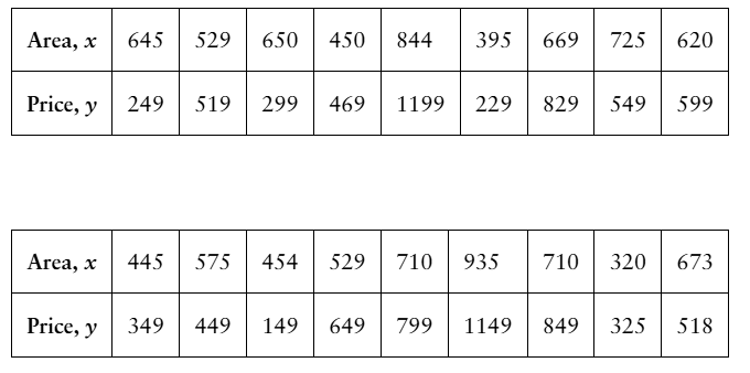
18. [APPLET] The table shows the cooking areas (in square inches) of 18 gas grills and their prices (in dollars). The regression equation is y = 1.501x - 341.501. (Source: Lowe's)
Problem 9.R.24
"In Exercises 19-24, construct the indicated prediction interval and interpret the results.
24. Construct a 99% prediction interval for the price of a gas grill in Exercise 18 with a usable cooking area of 900 square inches."
Problem 9.R.23
"In Exercises 19-24, construct the indicated prediction interval and interpret the results.
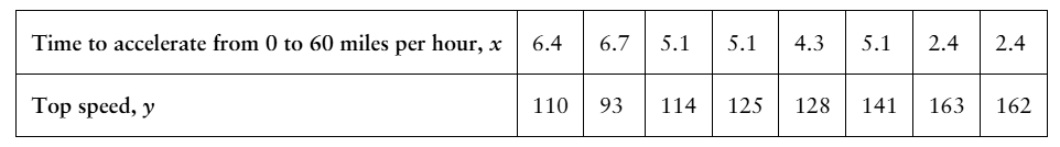
23. Construct a 99% prediction interval for the top speed of an electric car in Exercise 17 that takes 5.9 seconds to accelerate from 0 to 60 miles per hour."
Problem 9.R.20
"In Exercises 19-24, construct the indicated prediction interval and interpret the results.
20. Construct a 90% prediction interval for the average time adults ages 35 to 44 spend per day watching television in Exercise 10 when the average time adults ages 25 to 34 spend per day watching television is 2.25 hours."
Problem 9.R.19
"In Exercises 19-24, construct the indicated prediction interval and interpret the results.
19. Construct a 90% prediction interval for the amount of milk produced in Exercise 9 when there are an average of 9275 thousand milk cows."
Problem 9.R.27
"In Exercises 27 and 28, use the multiple regression equation to predict the y-values for the values of the independent variables.
27. An equation that can be used to predict fuel economy (in miles per gallon) for automobiles is
y=41.3- 0.004x_1 - 0.0049x_2
where x_1 is the engine displacement (in cubic inches) and x_2 is the vehicle weight (in
pounds).
a. x_1 = 305, x_2 = 3750
b. x_1 = 225, x_2 = 3100
c. x_1 = 105, x_2 = 2200
d. x_1 = 185, x_2 = 3000"
Problem 9.R.17
"In Exercises 17 and 18, use the data to (a) find the coefficient of determination r^2 and interpret
the result, and (b) find the standard error of estimate s_e and interpret the result.
17. The table shows the times (in seconds) to accelerate from 0 to 60 miles per hour and the top speeds (in miles per hour) for eight electric cars. The regression equation is y =- 14.399x + 196.996. (Source: Car and Driver)
Problem 9.R.22
"In Exercises 19-24, construct the indicated prediction interval and interpret the results.
22. Construct a 95% prediction interval for the fuel efficiency of an automobile in Exercise 12 that has an engine displacement of 265 cubic inches."
Problem 9.R.14
"In Exercises 13-16, use the value of the correlation coefficient r to calculate the coefficient of determination r^2. What does this tell you about the explained variation of the data about the regression line? about the unexplained variation?
14.r =- 0.937"
Problem 9.R.28
"In Exercises 27 and 28, use the multiple regression equation to predict the y-values for the values of the independent variables.
28. Use the regression equation found in Exercise 25.
a. x_1 = 9.0, x_2 = 0.70
b. x_1 = 3.0, x_2 = 0.25
c. x_1 = 8.0, x_2 = 0.60
d. x_1 = 5.2, x_2 = 0.46"
Problem 9.R.21
"In Exercises 19-24, construct the indicated prediction interval and interpret the results.
21. Construct a 95% prediction interval for the number of hours of sleep for an adult in Exercise 11 who is 45 years old."
Problem 9.RE.13
"In Exercises 13-16, use the value of the correlation coefficient r to calculate the coefficient of determination r^2. What does this tell you about the explained variation of the data about the regression line? about the unexplained variation?
13. r =- 0.450"
Problem 9.RE.15
"In Exercises 13-16, use the value of the correlation coefficient r to calculate the coefficient of determination r^2. What does this tell you about the explained variation of the data about the regression line? about the unexplained variation?
15. r = 0.642"
Problem 9.T.7a
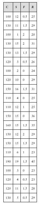
"The U.S. Food and Drug Administration (FDA) requires nutrition labeling for most foods. Un FDA regulations, manufacturers are required to list the amounts of certain nutrients in their foods, such as calories, sugar, fat, and carbohydrates. This nutritional information is displayed in the ""Nutrition Facts"" panel on the food's package.
The table shows the nutritional content below for one cup of each of 21 different breakfast
cereals.
C = calories
S = sugar in grams
F = fat in grams
R = carbohydrates in grams
7. Use the equations from Exercise 6 to predict the calories in 1 cup of cereal that has 7 grams of sugar, 0.5 gram of fat, and 31 grams of carbohydrates."
Problem 9.T.8
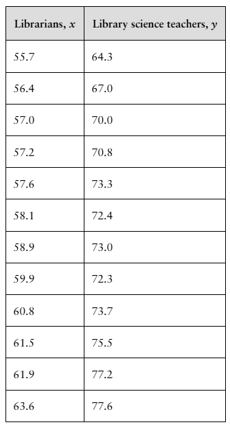
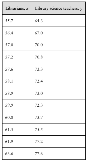
"[APPLET] For Exercises 2–9, use the data in the table, which shows the average annual salaries (both in thousands of dollars) for librarians and postsecondary library science teachers in the United States for 12 years. (Source: U.S. Bureau of Labor Statistics)
8. Find the standard error of estimate Se and interpret the result."
Problem 9.T.1
"1. Net Sales The equation used to predict the net sales (in millions of dollars) for a fiscal
year for a clothing retailer is y=23,769 + 9.18x_1 - 8.41x_2
where x_1 is the number of stores open at the end of the fiscal year and x_2 is the average
square footage per store. Use the multiple regression equation to predict the y-values for
the values of the independent variables.
a. x_1 = 1057, x_2 = 3698
b. x_1 = 1012, x_2 = 3659
c. x_1 = 952, x_2 = 3601
d. x_1 = 914, x_2 = 3594"
Problem 9.T.7
"[APPLET] For Exercises 2–9, use the data in the table, which shows the average annual salaries (both in thousands of dollars) for librarians and postsecondary library science teachers in the United States for 12 years. (Source: U.S. Bureau of Labor Statistics)
7. Find the coefficient of determination r^2 and interpret the result."
Problem 9.T.6
"[APPLET] For Exercises 2–9, use the data in the table, which shows the average annual salaries (both in thousands of dollars) for librarians and postsecondary library science teachers in the United States for 12 years. (Source: U.S. Bureau of Labor Statistics)
6. Use the regression equation that you found in Exercise 5 to predict the average annual salary of postsecondary library science teachers when the average annual salary of librarians is $61,000."
Problem 9.1.38a
Writing Use an appropriate research source to find a real-life data set with the indicated cause-and-effect relationship. Write a paragraph describing each variable and explain why you think the variables have the indicated cause-and-effect relationship.
a. Direct Cause-and-Effect: Changes in one variable cause changes in the other variable.
Problem 9.3.12a
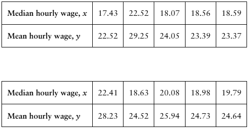
"Finding the Coefficient of Determination and the Standard Error of Estimate In Exercises 11-20, use the data to (a) find the coefficient of determination r^2 and interpret the result,
12. [APPLET] Median and Mean Hourly Wages The table shows the median and mean hourly wages (in dollars) in 10 states in a recent year. The equation of the regression line is y = 1.208x + 1.495. (Source: U.S. Census Bureau)
"
Problem 9.1.38b
Writing Use an appropriate research source to find a real-life data set with the indicated cause-and-effect relationship. Write a paragraph describing each variable and explain why you think the variables have the indicated cause-and-effect relationship.
b. Other Factors: The relationship between the variables is caused by a third variable.
Problem 9.3.12b
"Finding the Coefficient of Determination and the Standard Error of Estimate In Exercises 11-20, use the data to (b) find the standard error of estimate s_e and interpret the result.
12. [APPLET] Median and Mean Hourly Wages The table shows the median and mean hourly wages (in dollars) in 10 states in a recent year. The equation of the regression line is y = 1.208x + 1.495. (Source: U.S. Census Bureau)
"
Problem 9.1.38c
Writing Use an appropriate research source to find a real-life data set with the indicated cause-and-effect relationship. Write a paragraph describing each variable and explain why you think the variables have the indicated cause-and-effect relationship.
c. Coincidence: The relationship between the variables is a coincidence.