Back
BackProblem 10.3.26
Performing a Two-Sample F-Test In Exercises 19 –26, (a) identify the claim and state H0 and Ha, (b) find the critical value and identify the rejection region, (c) find the test statistic F, (d) decide whether to reject or fail to reject the null hypothesis, and (e) interpret the decision in the context of the original claim. Assume the samples are random and independent, and the populations are normally distributed.
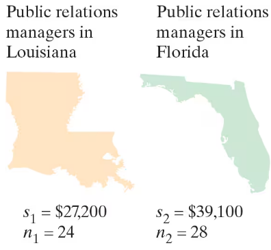
Annual Salaries An employment information service claims that the standard deviation of the annual salaries for public relations managers is less in Louisiana than in Florida. You select a sample of public relations managers from each state. The results of each survey are shown in the figure. At α=0.05, can you support the service’s claim? (Adapted from America’s Career InfoNet)
Problem 10.1.17
Testing for Normality Using a chi-square goodness-of-fit test, you can decide, with some degree of certainty, whether a variable is normally distributed. In all chi-square tests for normality, the null and alternative hypotheses are as listed below.
H₀: The variable has a normal distribution.
Hₐ: The variable does not have a normal distribution.
To determine the expected frequencies when performing a chi-square test for normality, first estimate the mean and standard deviation of the frequency distribution. Then, use the mean and standard deviation to compute the z-score for each class boundary. Then, use the z-scores to calculate the area under the standard normal curve for each class. Multiplying the resulting class areas by the sample size yields the expected frequency for each class.In Exercises 17 and 18, (a) find the expected frequencies, (b) find the critical value and identify the rejection region, (c) find the chi-square test statistic, (d) decide whether to reject or fail to reject the null hypothesis, and (e) interpret the decision in the context of the original claim.
In Exercises 17 and 18, (a) find the expected frequencies, (b) find the critical value and identify the rejection region, (c) find the chi-square test statistic, (d) decide whether to reject or fail to reject the null hypothesis, and (e) interpret the decision in the context of the original claim.
Test Scores At α=0.01, test the claim that the 200 test scores shown in the frequency distribution are normally distributed.
Problem 10.4.2
What conditions are necessary in order to use a one-way ANOVA test?
Problem 10.3.19
"Performing a Two-Sample F-Test In Exercises 19 –26, (a) identify the claim and state H0 and Ha, (b) find the critical value and identify the rejection region, (c) find the test statistic F, (d) decide whether to reject or fail to reject the null hypothesis, and (e) interpret the decision in the context of the original claim. Assume the samples are random and independent, and the populations are normally distributed.
Life of Appliances Company A claims that the variance of the lives of its appliances is less than the variance of the lives of Company B’s appliances. A sample of the lives of 20 of Company A’s appliances has a variance of 1.8. A sample of the lives of 25 of Company B’s appliances has a variance of 3.9. At α=0.025, can you support Company A’s claim?"
Problem 10.2.42
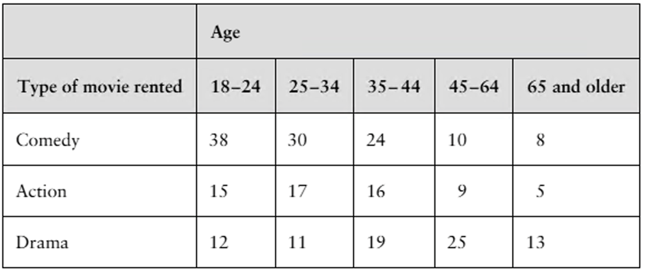
Conditional Relative Frequencies In Exercises 37 –42, use the contingency table from Exercises 33–36, and the information below.
Relative frequencies can also be calculated based on the row totals (by dividing each row entry by the row’s total) or the column totals (by dividing each column entry by the column’s total). These frequencies are conditional relative frequencies and can be used to determine whether an association exists between two categories in a contingency table.
What percent of U.S. adults ages 25 and over who are not high school graduates are unemployed?
Problem 10.2.4
Explain why the chi-square independence test is always a right-tailed test.
Problem 10.1.16
Performing a Chi-Square Goodness-of-Fit Test
In Exercises 7–16, (a) identify the claim and state H₀ and Hₐ, (b) find the critical value and identify the rejection region, (c) find the chi-square test statistic, (d) decide whether to reject or fail to reject the null hypothesis, and (e) interpret the decision in the context of the original claim.
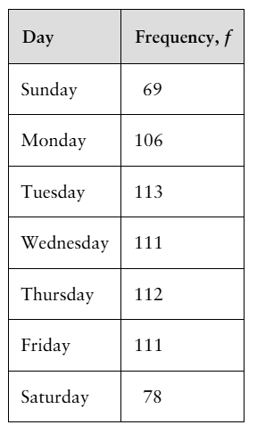
Births by Day of the Week A doctor claims that the number of births by day of the week is uniformly distributed. To test this claim, you randomly select 700 births from a recent year and record the day of the week on which each takes place. The table shows the results. At α=0.10, test the doctor’s claim. (Adapted from National Center for Health Statistics)
Problem 10.3.22
Performing a Two-Sample F-Test In Exercises 19 –26, (a) identify the claim and state H0 and Ha, (b) find the critical value and identify the rejection region, (c) find the test statistic F, (d) decide whether to reject or fail to reject the null hypothesis, and (e) interpret the decision in the context of the original claim. Assume the samples are random and independent, and the populations are normally distributed.
Heart Transplant Waiting Times The table at the left shows a sample of the waiting times (in days) for a heart transplant for two age groups. At α=0.05, can you conclude that the variances of the waiting times differ between the two age groups? (Adapted from Organ Procurement and Transplantation Network)
Problem 10.3.6
"Finding a Critical F-Value for a Right-Tailed Test In Exercises 5 – 8, find the critical F-value for a right-tailed test using the level of significance α and degrees of freedom d.f.N and d.f.D.
α=0.01, d.f.N=2, d.f.D=11"
Problem 10.3.8
"Finding a Critical F-Value for a Right-Tailed Test In Exercises 5 – 8, find the critical F-value for a right-tailed test using the level of significance α and degrees of freedom d.f.N and d.f.D.
α=0.025, d.f.N=7, d.f.D=3"
Problem 10.3.20
"Performing a Two-Sample F-Test In Exercises 19 –26, (a) identify the claim and state H0 and Ha, (b) find the critical value and identify the rejection region, (c) find the test statistic F, (d) decide whether to reject or fail to reject the null hypothesis, and (e) interpret the decision in the context of the original claim. Assume the samples are random and independent, and the populations are normally distributed.
Carbon Monoxide Emissions An automobile manufacturer claims that the variance of the carbon monoxide emissions for a make and model of one of its vehicles is less than the variance of the carbon monoxide emissions for a top competitor’s equivalent vehicle. A sample of the carbon monoxide emissions of 19 of the manufacturer’s specified vehicles has a variance of 0.008. A sample of the carbon monoxide emissions of 21 of its competitor’s equivalent vehicles has a variance of 0.045. At α=0.10, can you support the manufacturer’s claim? (Adapted from U.S. Environmental Protection Agency)"
Problem 10.3.14
"In Exercises 13 –18, test the claim about the difference between two population variances σ₁² and σ₂² at the level of significance α. Assume the samples are random and independent, and the populations are normally distributed.
Claim: σ₁² = σ₂²; α = 0.05.
Sample statistics: s₁² = 310, n₁ = 7 and s₂² = 297, n₂ = 8"
Problem 10.2.12
Finding Expected Frequencies
In Exercises 7–12, (a) calculate the marginal frequencies and (b) find the expected frequency for each cell in the contingency table. Assume that the variables are independent.
Problem 10.3.9
Finding a Critical F-Value for a Two-Tailed Test In Exercises 9 –12, find the critical F-value for a two-tailed test using the level of significance α and degrees of freedom d.f.N and d.f.D.
α=0.01, d.f.N=6, d.f.D=7
Problem 10.4.13
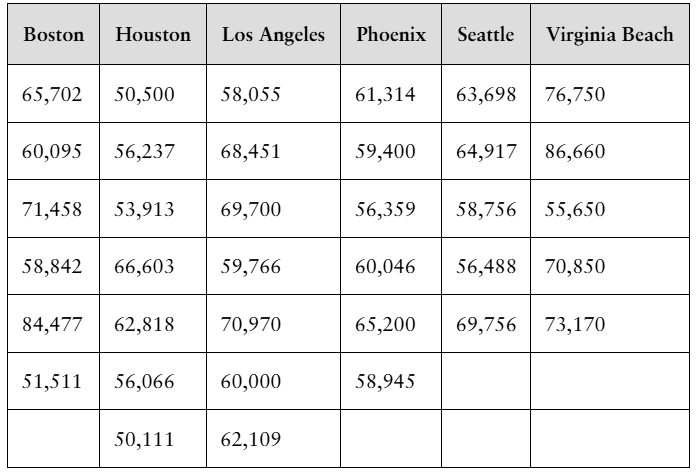
Performing a One-Way ANOVA Test In Exercises 5 –14, (a) identify the claim and state H0 and Ha, (b) find the critical value and identify the rejection region, (c) find the test statistic F, (d) decide whether to reject or fail to reject the null hypothesis, and (e) interpret the decision in the context of the original claim. Assume the samples are random and independent, the populations are normally distributed, and the population variances are equal.
[APPLET] Statistician Salaries The table shows the salaries of a sample of entry level statisticians from six large metropolitan areas. At α=0.05, can you conclude that the mean salary is different in at least one of the areas? (Adapted from Salary.com)
Problem 10.2.28
Performing a Chi-Square Independence Test In Exercises 13–28, perform the indicated chi-square independence test by performing the steps below.
a. Identify the claim and state H₀ and Hₐ
b. Determine the degrees of freedom, find the critical value, and identify the rejection region.
c. Find the chi-square test statistic.
d. Decide whether to reject or fail to reject the null hypothesis.
e. Interpret the decision in the context of the original claim.
Use the contingency table and expected frequencies from Exercise 11. At α=0.10, test the hypothesis that the variables are independent.
Problem 10.3.1
Explain how to find the critical value for an F-test.
Problem 10.3.11
"Finding a Critical F-Value for a Two-Tailed Test In Exercises 9 –12, find the critical F-value for a two-tailed test using the level of significance α and degrees of freedom d.f.N and d.f.D.
α=0.05, d.f.N=60, d.f.D=40"
Problem 10.2.20
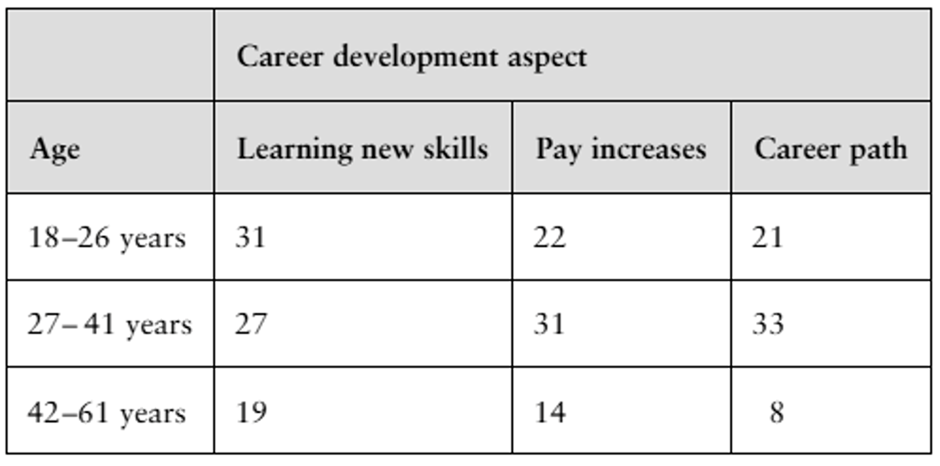
Performing a Chi-Square Independence Test In Exercises 13–28, perform the indicated chi-square independence test by performing the steps below.
a. Identify the claim and state H₀ and Hₐ
b. Determine the degrees of freedom, find the critical value, and identify the rejection region.
c. Find the chi-square test statistic.
d. Decide whether to reject or fail to reject the null hypothesis.
e. Interpret the decision in the context of the original claim.
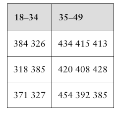
Ages and Goals You are investigating the relationship between the ages of U.S. adults and what aspect of career development they consider to be the most important. You randomly collect the data shown in the contingency table. At α=0.10, is there enough evidence to conclude that age is related to which aspect of career development is considered to be most important? (Adapted from The Harris Poll)
Problem 10.2.36
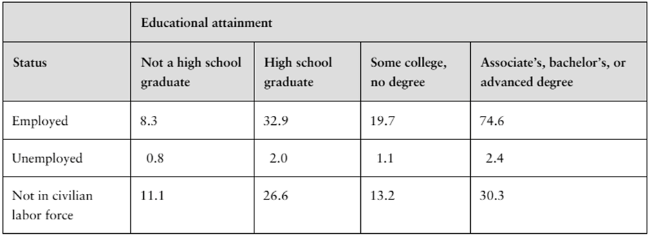
Contingency Tables and Relative Frequencies In Exercises 33–36, use the information below.
The frequencies in a contingency table can be written as relative frequencies by dividing each frequency by the sample size. The contingency table below shows the number of U.S. adults (in millions) ages 25 and over by employment status and educational attainment. (Adapted from U.S. Census Bureau)
What percent of U.S. adults ages 25 and over (a) are employed and are only high school graduates, (b) are not in the civilian labor force, and (c) are not high school graduates?
Problem 10.3.5
"Finding a Critical F-Value for a Right-Tailed Test In Exercises 5 – 8, find the critical F-value for a right-tailed test using the level of significance α and degrees of freedom d.f.N and d.f.D.
α=0.05, d.f.N=9, d.f.D=16"
Problem 10.4.11
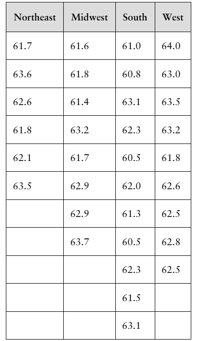
Performing a One-Way ANOVA Test In Exercises 5 –14, (a) identify the claim and state H0 and Ha, (b) find the critical value and identify the rejection region, (c) find the test statistic F, (d) decide whether to reject or fail to reject the null hypothesis, and (e) interpret the decision in the context of the original claim. Assume the samples are random and independent, the populations are normally distributed, and the population variances are equal.
[APPLET] Well-Being Index The well-being index is a way to measure how people are faring physically, emotionally, socially, and professionally, as well as to rate the overall quality of their lives and their outlooks for the future. The table shows the well-being index scores for a sample of states from four regions of the United States. At α=0.10, can you reject the claim that the mean score is the same for all regions? (Adapted from Gallup and Healthways)
Problem 10.2.22
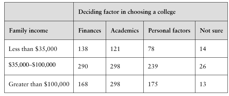
Performing a Chi-Square Independence Test In Exercises 13–28, perform the indicated chi-square independence test by performing the steps below.
a. Identify the claim and state H₀ and Hₐ
b. Determine the degrees of freedom, find the critical value, and identify the rejection region.
c. Find the chi-square test statistic.
d. Decide whether to reject or fail to reject the null hypothesis.
e. Interpret the decision in the context of the original claim.
Choosing a College The contingency table shows the results of a survey asking 1858 parents and students of different incomes what their deciding factor was in choosing a college. At α=0.01, can you conclude that the deciding factor in choosing a college is related to the income of the family? (Adapted from Sallie Mae)
Problem 10.2.6
True or False? In Exercises 5 and 6, determine whether the statement is true or false. If it is false, rewrite it as a true statement.
When the test statistic for the chi-square independence test is large, you will, in most cases, reject the null hypothesis.
Problem 10.4.4
Describe the hypotheses for a two-way ANOVA test.
Problem 10.1.4
Finding Expected Frequencies
In Exercises 3 – 6, find the expected frequency for the values of n and pᵢ.
n=500, pᵢ=0.9
Problem 10.3.28
"Finding Left-Tailed Critical F-Values In this section, you only needed to calculate the right-tailed critical F-value for a two-tailed test. For other applications of the F-distribution, you will need to calculate the left-tailed critical F-value. To calculate the left-tailed critical F-value, perform the steps below.
1. Interchange the values for d.f.N and d.f.D.
2. Find the corresponding F-value in Table 7.
3. Calculate the reciprocal of the F-value to obtain the left-tailed critical F-value.
In Exercises 27 and 28, find the right- and left-tailed critical F-values for a two-tailed test using the level of significance α and degrees of freedom d.f.N and d.f.D.
α=0.10, d.f.N=20, d.f.D=15"
Problem 10.1.12
Performing a Chi-Square Goodness-of-Fit Test
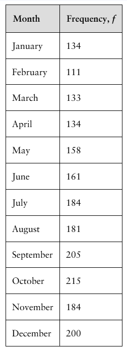
In Exercises 7–16, (a) identify the claim and state H₀ and Hₐ, (b) find the critical value and identify the rejection region, (c) find the chi-square test statistic, (d) decide whether to reject or fail to reject the null hypothesis, and (e) interpret the decision in the context of the original claim.
Homicides by Month A researcher claims that the number of homicide crimes in California by month is uniformly distributed. To test this claim, you randomly select 2000 homicides from a recent year and record the month when each happened. The table shows the results. At α=0.10, test the researcher’s claim. (Adapted from California Department of Justice)
Problem 10.1.18
Testing for Normality Using a chi-square goodness-of-fit test, you can decide, with some degree of certainty, whether a variable is normally distributed. In all chi-square tests for normality, the null and alternative hypotheses are as listed below.
H₀: The variable has a normal distribution.
Hₐ: The variable does not have a normal distribution.
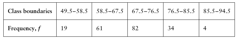
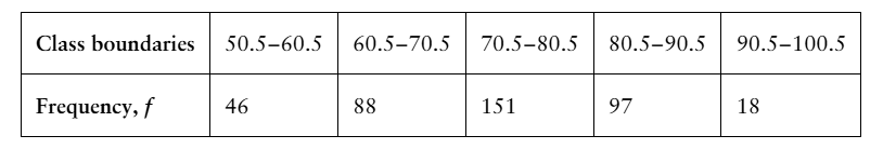
To determine the expected frequencies when performing a chi-square test for normality, first estimate the mean and standard deviation of the frequency distribution. Then, use the mean and standard deviation to compute the z-score for each class boundary. Then, use the z-scores to calculate the area under the standard normal curve for each class. Multiplying the resulting class areas by the sample size yields the expected frequency for each class.In Exercises 17 and 18, (a) find the expected frequencies, (b) find the critical value and identify the rejection region, (c) find the chi-square test statistic, (d) decide whether to reject or fail to reject the null hypothesis, and (e) interpret the decision in the context of the original claim.
In Exercises 17 and 18, (a) find the expected frequencies, (b) find the critical value and identify the rejection region, (c) find the chi-square test statistic, (d) decide whether to reject or fail to reject the null hypothesis, and (e) interpret the decision in the context of the original claim.
Test Scores At α=0.05, test the claim that the 400 test scores shown in the frequency distribution are normally distributed.
Problem 10.3.12
"Finding a Critical F-Value for a Two-Tailed Test In Exercises 9 –12, find the critical F-value for a two-tailed test using the level of significance α and degrees of freedom d.f.N and d.f.D.
α=0.05, d.f.N=27, d.f.D=19"