Young Adults In a survey of 3500 males ages 20 to 24 whose highest level of education is some college, but no bachelor’s degree, 80.2% were employed. In a survey of 2000 males ages 20 to 24 whose highest level of education is a bachelor’s degree or higher, 86.4% were employed. At α=0.01, can you support the claim that there is a difference in the proportion of those employed between the two groups? (Adapted from National Center for Education Statistics)

What conditions are necessary to use the dependent samples t-test for the mean of the differences for a population of paired data?

Testing a Difference Other Than Zero Sometimes a researcher is interested in testing a difference in means other than zero. In Exercises 27 and 28, you will test the difference between two means using a null hypothesis of Ho: μ1-μ2=k, Ho: μ1-μ2>=k or Ho: μ1-μ2<=k . The standardized test statistic is still

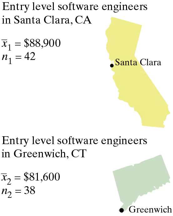
Software Engineer Salaries Is the difference between the mean annual salaries of entry level software engineers in Santa Clara, California, and Greenwich, Connecticut, more than $4000? To decide, you select a random sample of entry level software engineers from each city. The results of each survey are shown in the figure at the left. Assume the population standard deviations are σ1=$14,060 and σ2=$13,050 . At α=0.05, what should you conclude? (Adapted from Salary.com)

Blue Crabs A marine researcher claims that the stomachs of blue crabs from one location contain more fish than the stomachs of blue crabs from another location. The stomach contents of a sample of 25 blue crabs from Location A contain a mean of 320 milligrams of fish and a standard deviation of 60 milligrams. The stomach contents of a sample of 15 blue crabs from Location B contain a mean of 280 milligrams of fish and a standard deviation of 80 milligrams. At , α= 0.01can you support the marine researcher’s claim? Assume the population variances are equal.

Testing the Difference Between Two Proportions In Exercises 7–12, (a) identify the claim and state Ho and Ha, (b) find the critical value(s) and identify the rejection region(s), (c) find the standardized test statistic z, (d) decide whether to reject or fail to reject the null hypothesis, and (e) interpret the decision in the context of the original claim. Assume the samples are random and independent.

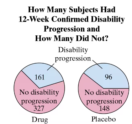
Multiple Sclerosis Drug In a study to determine the effectiveness of using a drug to treat multiple sclerosis, 488 subjects were given the drug and 244 subjects were given a placebo. The numbers of subjects who had 12-week confirmed disability progression were tracked. The results are shown at the left. At α=0.01, can you support the claim that there is a difference in the proportion of subjects who had no 12-week confirmed disability progression? (Adapted from The New England Journal of Medicine)

In Exercises 11 –14, test the claim about the difference between two population means and at the level of significance . Assume the samples are random and independent, and the populations are normally distributed.

Claim: μ1<μ2; α=0.03

Population statistics:σ1=136 and σ2=215

Sample Statistics: x̅1=5004, n1=144, x̅2=4895, n2=156

Testing the Difference Between Two Means In Exercises 15–24, (a) identify the claim and state Ho and Ha, (b) find the critical value(s) and identify the rejection region(s), (c) find the standardized test statistic z, (d) decide whether to reject or fail to reject the null hypothesis, and (e) interpret the decision in the context of the original claim. Assume the samples are random and independent, and the populations are normally distributed.

ACT Mathematics and Science Scores The mean ACT mathematics score for 60 high school students is 20.2. Assume the population standard deviation is 5.7. The mean ACT science score for 75 high school students is 20.6. Assume the population standard deviation is 5.9. At α=0.01, can you reject the claim that ACT mathematics and science scores are equal? (Source: ACT, Inc.)

Testing the Difference Between Two Means, (a) identify the claim and state H0 and Ha , (b) find the critical value(s) and identify the rejection region(s), (c) find the standardized test statistic t, (d) decide whether to reject or fail to reject the null hypothesis, and (e) interpret the decision in the context of the original claim. Assume the samples are random and independent, and the populations are normally distributed.

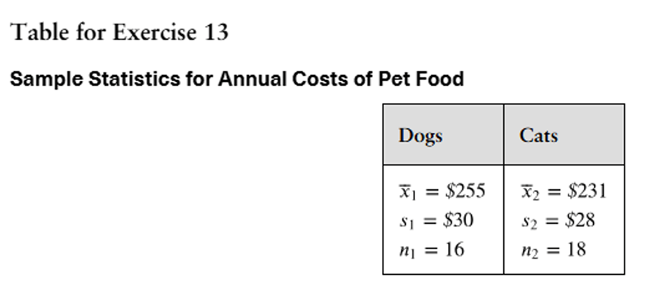
Pet Food

A pet association claims that the mean annual costs of food for dogs and cats are the same. The results for samples of the two types of pets are shown at the left. At , α=0.10 can you reject the pet association’s claim? Assume the population variances are equal. (Adapted from American Pet Products Association)

[APPLET] Teaching Methods

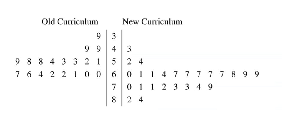
A new method of teaching reading is being tested on third grade students. A group of third grade students is taught using the new curriculum. A control group of third grade students is taught using the old curriculum. The reading test scores for the two groups are shown in the back-to-back stem-and-leaf plot.

At , α=0.10 is there enough evidence to support the claim that the new method of teaching reading produces higher reading test scores than the old method does? Assume the population variances are equal.

What conditions are necessary in order to use the z-test to test the difference between two population means?

[APPLET] Teaching Methods

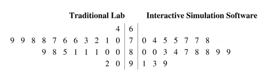
Two teaching methods and their effects on science test scores are being reviewed. A group of students is taught in traditional lab sessions. A second group of students is taught using interactive simulation software. The science test scores for the two groups are shown in the back-to-back stem-and-leaf plot.

At , α=0.01 can you support the claim that the mean science test score is lower for students taught using the traditional lab method than it is for students taught using the interactive simulation software? Assume the population variances are equal.

Testing the Difference Between Two Means In Exercises 15–24, (a) identify the claim and state Ho and Ha, (b) find the critical value(s) and identify the rejection region(s), (c) find the standardized test statistic z, (d) decide whether to reject or fail to reject the null hypothesis, and (e) interpret the decision in the context of the original claim. Assume the samples are random and independent, and the populations are normally distributed.

Braking Distances To compare the dry braking distances from 60 to 0 miles per hour for two makes of automobiles, a safety engineer conducts braking tests for 16 compact SUVs and 11 midsize SUVs. The mean braking distance for the compact SUVs is 131.8 feet. Assume the population standard deviation is 5.5 feet. The mean braking distance for the midsize SUVs is 132.8 feet. Assume the population standard deviation is 6.7 feet. At α=0.10 , can the engineer support the claim that the mean braking distances are different for the two categories of SUVs? (Adapted from Consumer Reports)

Test the claim about the mean of the differences for a population of paired data at the level of significance α. Assume the samples are random and dependent, and the populations are normally distributed.

Claim: μd<0 , α=0.05 , Sample statistics: d̄ =1.5 , sd=3.2 , n=14

Test the claim about the difference between two population means and at the level of significance α. Assume the samples are random and independent, and the populations are normally distributed.

Claim: μ1<μ2, α=0.10, Assume (σ1)^2=(σ2)^2

Sample statistics:

x̅1=0.345, s1=0.305 , n1=11 and x̅2=0.515, s2=0.215, n2=9

In Exercises 11 –14, test the claim about the difference between two population means and at the level of significance . Assume the samples are random and independent, and the populations are normally distributed.

Claim: μ1>μ2; α=0.10

Population statistics:σ1=40 and σ2=15

Sample Statistics: x̅1=500, n1=100, x̅2=495, n2=75

Test the claim about the difference between two population means and at the level of significance α. Assume the samples are random and independent, and the populations are normally distributed.

Claim: μ1=μ2, α=0.01, Assume (σ1)^2=(σ2)^2

Test the claim about the difference between two population means and at the level of significance α. Assume the samples are random and independent, and the populations are normally distributed.

Claim: μ1≤μ2, α=0.05, Assume (σ1)^2≠(σ2)^2

Sample statistics:

x̅1=2410, s1=175, n1=13 and x̅2=2305, s2=52, n2=10

Independent and Dependent Samples In Exercises 5– 8, classify the two samples as independent or dependent and justify your answer.

Sample 1: The IQ scores of 60 females

Sample 2: The IQ scores of 60 males

In Exercises 3 – 6, determine whether a normal sampling distribution can be used. If it can be used, test the claim about the difference between two population proportions and at the level of significance . Assume the samples are random and independent.

Claim: p1≠p2, α=0.01

Sample statistics: x1=35, n1=70, and x2=36, n2=60

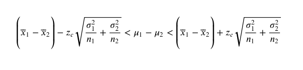
Constructing Confidence Intervals for p1-p2 You can construct a confidence interval for the difference between two population proportions p1-p2 by using the inequality below.

[Image] Complicated mathematical formula.

In Exercises 23–26, construct the indicated confidence interval for p1-p2. Assume the samples are random and independent.

Critical Threats Repeat Exercise 25 but with a 99% confidence interval. Describe the likelihood that equal proportions of the population see cyberterrorism and the spread of infectious diseases as critical threats in the next 10 years.

Explain how to perform a two-sample z-test for the difference between two population means using independent samples with and known.

What conditions are necessary to use the t-test for testing the difference between two population means?

Test the claim about the difference between two population means and at the level of significance α. Assume the samples are random and independent, and the populations are normally distributed.

Claim: μ1>μ2, α=0.01, Assume (σ1)^2≠(σ2)^2 

Sample statistics:

x̅1=52, s1=4.8, n1=32 and x̅2=50, s2=1.2, n2=40

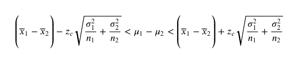
Constructing Confidence Intervals for μ1-μ2. You can construct a confidence interval for the difference between two population means μ1-μ2 , as shown below, when both population standard deviations are known, and either both populations are normally distributed or both n1>= 30 and n2>=30 . Also, the samples must be randomly selected and independent.

[Image]

In Exercises 29 and 30, construct the indicated confidence interval for μ1-μ2 .

Software Engineer Salaries Construct a 95% confidence interval for the difference between the mean annual salaries of entry level software engineers in Santa Clara, California, and Greenwich, CT, using the data from Exercise 27.

Testing the Difference Between Two Means In Exercises 15–24, (a) identify the claim and state Ho and Ha, (b) find the critical value(s) and identify the rejection region(s), (c) find the standardized test statistic z, (d) decide whether to reject or fail to reject the null hypothesis, and (e) interpret the decision in the context of the original claim. Assume the samples are random and independent, and the populations are normally distributed.

ACT English and Reading Scores The mean ACT English score for 120 high school students is 19.9. Assume the population standard deviation is 7.2. The mean ACT reading score for 150 high school students is 21.2. Assume the population standard deviation is 7.1. At α=0.10, can you support the claim that ACT reading scores are higher than ACT English scores? (Source: ACT, Inc.)

Independent and Dependent Samples In Exercises 5– 8, classify the two samples as independent or dependent and justify your answer.

Sample 1: The maximum bench press weights for 53 football players

Sample 2: The maximum bench press weights for the same 53 football players after completing a weight lifting program

Yellowfin Tuna

A marine biologist claims that the mean fork length (see figure at the left) of yellowfin tuna is different in two zones in the eastern tropical Pacific Ocean. A sample of 26 yellowfin tuna collected in Zone A has a mean fork length of 76.2 centimeters and a standard deviation of 16.5 centimeters. A sample of 31 yellowfin tuna collected in Zone B has a mean fork length of 80.8 centimeters and a standard deviation of 23.4 centimeters. At ,α=0.01 can you support the marine biologist’s claim? Assume the population variances are equal. (Adapted from Fishery Bulletin)

Testing a Difference Other Than Zero Sometimes a researcher is interested in testing a difference in means other than zero. In Exercises 27 and 28, you will test the difference between two means using a null hypothesis of Ho: μ1-μ2=k, Ho: μ1-μ2>=k or Ho: μ1-μ2<=k . The standardized test statistic is still

Architect Salaries Is the difference between the mean annual salaries of entry level architects in Denver, Colorado, and Lincoln, Nebraska, equal to $9000? To decide, you select a random sample of entry level architects from each city. The results of each survey are shown in the figure. Assume the population standard deviations are σ1=$6560 and σ2=$6100 . At α=0.01 what should you conclude? (Adapted from Salary.com)

Constructing Confidence Intervals for μ1-μ2. You can construct a confidence interval for the difference between two population means μ1-μ2 , as shown below, when both population standard deviations are known, and either both populations are normally distributed or both n1>= 30 and n2>=30 . Also, the samples must be randomly selected and independent.

In Exercises 29 and 30, construct the indicated confidence interval for μ1-μ2 .

Architect Salaries Construct a 99% confidence interval for the difference between the mean annual salaries of entry level architects in Denver, Colorado, and Lincoln, Nebraska, using the data from Exercise 28.

Find the critical value(s) for the alternative hypothesis, level of significance , and sample sizes and . Assume that the samples are random and independent, the populations are normally distributed, and the population variances are (a) equal and (b) not equal.

Ha:μ1>μ2 , α=0.01 , n1=12 , n2=15