Estimating the Median Use the sample data listed in Exercise 1 “Bootstrap Requirements” to generate 1000 bootstrap samples, and find the median in each of those samples. After obtaining the 1000 sample medians, find the 95% confidence interval estimate of the population median by evaluating p2.5 and p97.5 from the sorted 1000 medians. Given that the sample times in Exercise 1 are from the 50 times in Data Set 20 “Alcohol and Tobacco in Movies” and those 50 times have a median of 5.5, how well did the bootstrap method work to create a “good” confidence interval?
Table of contents
- 1. Intro to Stats and Collecting Data1h 14m
- 2. Describing Data with Tables and Graphs1h 56m
- 3. Describing Data Numerically2h 5m
- 4. Probability2h 16m
- 5. Binomial Distribution & Discrete Random Variables3h 6m
- 6. Normal Distribution and Continuous Random Variables2h 11m
- 7. Sampling Distributions & Confidence Intervals: Mean3h 23m
- Sampling Distribution of the Sample Mean and Central Limit Theorem19m
- Distribution of Sample Mean - Excel23m
- Introduction to Confidence Intervals15m
- Confidence Intervals for Population Mean1h 18m
- Determining the Minimum Sample Size Required12m
- Finding Probabilities and T Critical Values - Excel28m
- Confidence Intervals for Population Means - Excel25m
- 8. Sampling Distributions & Confidence Intervals: Proportion2h 10m
- 9. Hypothesis Testing for One Sample5h 8m
- Steps in Hypothesis Testing1h 6m
- Performing Hypothesis Tests: Means1h 4m
- Hypothesis Testing: Means - Excel42m
- Performing Hypothesis Tests: Proportions37m
- Hypothesis Testing: Proportions - Excel27m
- Performing Hypothesis Tests: Variance12m
- Critical Values and Rejection Regions28m
- Link Between Confidence Intervals and Hypothesis Testing12m
- Type I & Type II Errors16m
- 10. Hypothesis Testing for Two Samples5h 37m
- Two Proportions1h 13m
- Two Proportions Hypothesis Test - Excel28m
- Two Means - Unknown, Unequal Variance1h 3m
- Two Means - Unknown Variances Hypothesis Test - Excel12m
- Two Means - Unknown, Equal Variance15m
- Two Means - Unknown, Equal Variances Hypothesis Test - Excel9m
- Two Means - Known Variance12m
- Two Means - Sigma Known Hypothesis Test - Excel21m
- Two Means - Matched Pairs (Dependent Samples)42m
- Matched Pairs Hypothesis Test - Excel12m
- Two Variances and F Distribution29m
- Two Variances - Graphing Calculator16m
- 11. Correlation1h 24m
- 12. Regression3h 33m
- Linear Regression & Least Squares Method26m
- Residuals12m
- Coefficient of Determination12m
- Regression Line Equation and Coefficient of Determination - Excel8m
- Finding Residuals and Creating Residual Plots - Excel11m
- Inferences for Slope31m
- Enabling Data Analysis Toolpak1m
- Regression Readout of the Data Analysis Toolpak - Excel21m
- Prediction Intervals13m
- Prediction Intervals - Excel19m
- Multiple Regression - Excel29m
- Quadratic Regression15m
- Quadratic Regression - Excel10m
- 13. Chi-Square Tests & Goodness of Fit2h 21m
- 14. ANOVA2h 28m
7. Sampling Distributions & Confidence Intervals: Mean
Introduction to Confidence Intervals
Problem 7.3.14
Textbook Question
Mint Specs Listed below are weights (grams) from a simple random sample of pennies produced after 1983 (from Data Set 40 “Coin Weights” in Appendix B). Construct a 95% confidence interval estimate of for the population of such pennies. What does the confidence interval suggest about the U.S. Mint specifications that now require a standard deviation of 0.0230 g for weights of pennies?

 Verified step by step guidance
1
Step 1: Calculate the sample mean (\( \bar{x} \)) using the formula \( \bar{x} = \frac{\sum x_i}{n} \), where \( x_i \) are the individual weights and \( n \) is the sample size. Add all the weights provided and divide by the total number of weights.
Step 2: Calculate the sample standard deviation (\( s \)) using the formula \( s = \sqrt{\frac{\sum (x_i - \bar{x})^2}{n-1}} \). Subtract the sample mean from each weight, square the result, sum these squared differences, divide by \( n-1 \), and take the square root.
Step 3: Determine the critical value (\( t \)) for a 95% confidence interval using a t-distribution table. The degrees of freedom (df) are \( n-1 \), where \( n \) is the sample size.
Step 4: Compute the margin of error (ME) using the formula \( ME = t \cdot \frac{s}{\sqrt{n}} \), where \( s \) is the sample standard deviation and \( n \) is the sample size.
Step 5: Construct the confidence interval using the formula \( \text{Confidence Interval} = \bar{x} \pm ME \). Interpret the interval in the context of the U.S. Mint specifications, comparing the calculated standard deviation to the required standard deviation of 0.0230 g.
 Verified video answer for a similar problem:
This video solution was recommended by our tutors as helpful for the problem above
Video duration:
8mPlay a video:
0 Comments
Key Concepts
Here are the essential concepts you must grasp in order to answer the question correctly.
Confidence Interval
A confidence interval is a range of values, derived from sample statistics, that is likely to contain the population parameter with a specified level of confidence, typically 95%. It is calculated using the sample mean, the standard deviation, and the sample size, providing a measure of uncertainty around the estimate. For example, if the confidence interval for the mean weight of pennies is (2.490, 2.510), we can be 95% confident that the true mean weight lies within this range.
Recommended video:

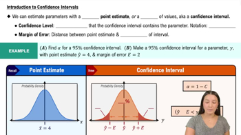
Introduction to Confidence Intervals
Standard Deviation
Standard deviation is a statistic that measures the dispersion or variability of a set of values. It indicates how much individual data points differ from the mean of the dataset. In the context of the U.S. Mint specifications, a standard deviation of 0.0230 grams suggests that the weights of the pennies produced are expected to vary by this amount from the average weight, which is crucial for quality control in manufacturing.
Recommended video:
Guided course

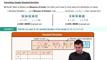
Calculating Standard Deviation
Simple Random Sample
A simple random sample is a subset of individuals chosen from a larger population, where each individual has an equal chance of being selected. This method helps ensure that the sample is representative of the population, reducing bias in statistical analysis. In this case, the weights of the pennies were collected from a simple random sample, allowing for valid inferences about the entire population of pennies produced after 1983.
Recommended video:

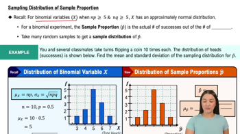
Sampling Distribution of Sample Proportion

 6:33m
6:33mWatch next
Master Introduction to Confidence Intervals with a bite sized video explanation from Patrick
Start learningRelated Videos
Related Practice
Textbook Question
