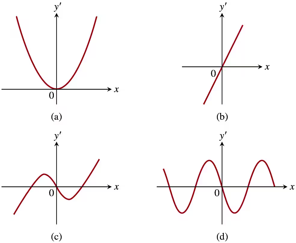
Match the functions graphed in Exercises 27–30 with the derivatives graphed in the accompanying figures (a)–(d).
Verified step by step guidance
1
Step 1: Analyze the graph of the function y = f₁(x). The graph is a parabola opening upwards, which suggests that the function is quadratic, such as y = x².
Step 2: Recall that the derivative of a quadratic function y = x² is linear, specifically y' = 2x. This means the derivative graph will be a straight line passing through the origin.
Step 3: Compare the derivative graphs (a)-(d) provided. The graph labeled (b) is a straight line passing through the origin, which matches the derivative of y = x².
Step 4: Match the function y = f₁(x) with its derivative graph (b), as the characteristics align: quadratic function leads to a linear derivative.
Step 5: Verify the match by considering the slope of the derivative graph (b). The slope corresponds to the rate of change of the original function, confirming the relationship between y = f₁(x) and its derivative.
Verified video answer for a similar problem:
This video solution was recommended by our tutors as helpful for the problem above
Video duration:
3m
Play a video:
0 Comments
Key Concepts
Here are the essential concepts you must grasp in order to answer the question correctly.
Derivative and Slope
The derivative of a function at a point is the slope of the tangent line to the graph of the function at that point. It provides the rate of change of the function's value with respect to changes in the input. Understanding how the slope changes across the graph helps in matching functions to their derivatives, as the derivative graph represents these slopes.
Critical points occur where the derivative is zero or undefined, indicating potential maxima, minima, or inflection points. The sign of the derivative (positive or negative) indicates whether the function is increasing or decreasing. Analyzing these aspects helps in identifying the corresponding derivative graph, as changes in sign reflect changes in the function's behavior.
Graphically, the derivative of a function is represented as a new graph that shows the slope of the original function at each point. For example, a linear function's derivative is constant, while a quadratic function's derivative is linear. Recognizing these patterns is crucial for matching a function to its derivative graph, as each function type has a distinct derivative shape.


 Verified step by step guidance
 05:13
05:13