13. Intro to Differential Equations
Slope Fields
Struggling with Calculus?
Join thousands of students who trust us to help them ace their exams!Watch the first videoMultiple Choice
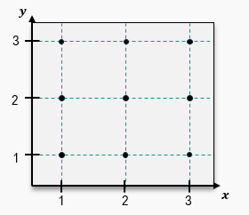
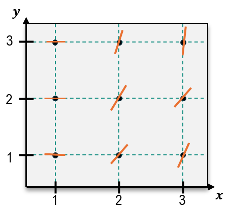
Sketch a slope field for the following differential equation through the nine points shown on the graph.
A
B
C
D
 Verified step by step guidance
1
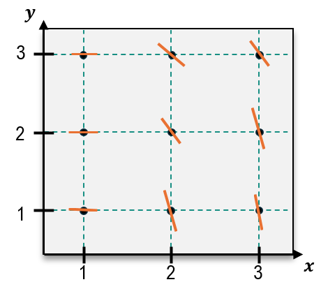
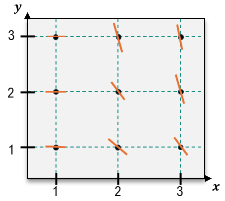
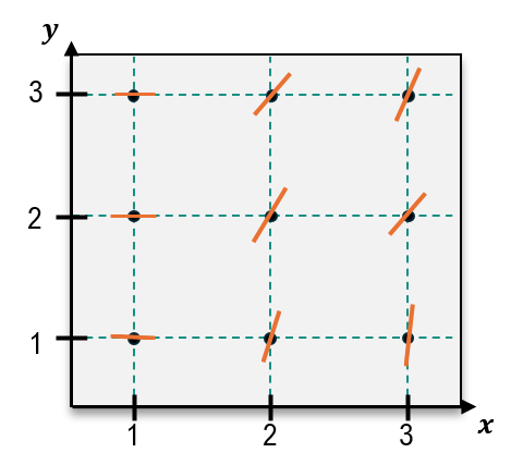
Step 1: Understand the problem. The goal is to sketch a slope field for the differential equation y′ = y − x through the nine points shown on the graph. A slope field visually represents the slope of the solution curve at various points in the plane.
Step 2: Recall that the slope at each point (x, y) is determined by substituting the coordinates of the point into the differential equation y′ = y − x. For example, at the point (1, 3), the slope is calculated as y′ = 3 − 1 = 2.
Step 3: Calculate the slope for each of the nine points on the graph. Substitute the x and y values of each point into the equation y′ = y − x. For instance, at (2, 2), the slope is y′ = 2 − 2 = 0, and at (3, 1), the slope is y′ = 1 − 3 = -2.
Step 4: Draw a small line segment at each point to represent the slope. The orientation of the line segment corresponds to the calculated slope. For example, a positive slope will tilt upwards, a negative slope will tilt downwards, and a slope of zero will be horizontal.
Step 5: Repeat this process for all nine points on the graph, ensuring that the slope field accurately represents the behavior of the differential equation y′ = y − x at each point.

 5:45m
5:45mWatch next
Master Understanding Slope Fields with a bite sized video explanation from Patrick
Start learningRelated Videos
0